Data Science, amongst other things.

Category: Guide

Building a Search Engine for E-Commerce with Elasticsearch

This is a continuation of my previous post on search engines. Having been involved with using Elasticsearch to build a search engine for e-commerce, there are some interesting ideas which I have taken away from the experience. I will go through some of the design decisions made and problems encountered along the way.

Tweaking the Search Query
Elasticsearch provides a huge variety of different query types, each of which has a different approach to retrieving search results. For example, the term query will find documents containing a certain term, the fuzzy query will match documents containing terms which are approximately equal to a given term, the geo-shape query enables you to perform useful queries over documents containing longitude and latitude coordinates and many more. Any of these query types can be composed using compositional query types, such as the bool query.

When I talk about tweaking the search query, I mean choosing the query types to use and structuring our query in a way that will enable us to achieve optimal results for any kind of search over the product base. The two main properties of the search query which we are trying to optimise are:

  1. How to best determine which products match
  2. How to best determine the order (i.e. relative importance) of the matching products

One of the first options that we considered using was the query-string query: a query type that parses your query and decides what query types to use, and often does the sensible thing. For instance, jeans will match any document containing the term jeans, blue jeans will match any document containing both ‘blue’ and ‘jeans’ and "blue jeans" will match documents containing both terms together (an exact match). You can even make more complex searches, like blue jeans -(levi OR diesel) which will match documents containing ‘blue’ and ‘jeans’ but not the terms ‘levi’ or ‘diesel’. This all seems quite nice at first, but this query type can give very unexpected results if used incorrectly – for example t-shirt will match documents containing ‘t’, but will exclude all documents containing ‘shirt’. Of course, customers can’t be expected to understand why this happens or how to fix their query.

Another option is the multi-match query, which takes a list of fields to query over and builds a sequence of match queries. Similar to the query-string query, each field can each be given a different boost factor, which is used in determining relative importance of some terms matching a given field. You can also tweak the type of multi_match – e.g. whether the query terms must all be found in a single field, or can be found in different fields (but not necessarily in the same field). Here is an example of a multi_match query:

{
  "multi_match" : {
    "query":      "gladiator russell crowe",
    "type":       "best_fields",
    "fields":     [ "title^10", "actors^5", "description^1" ]
  }
}

Here, we have used the boost operator (^) to indicate that the title field should be given the most importance. The query will still be matched against the description field, but matches in the title and actors fields will be given a higher score and will appear first in our result set. The best_fields type gives precedence when the query terms appear in the same field, but they don’t have to.

When matching across multiple fields, it can be tricky to figure out which documents are most relevant to the query. If we just consider which fields matched the query, then we won’t get optimal results. For example, if the query is ps4 controller and a document contains ‘ps4’ in the title field and ‘controller’ in the description field, then should it be given a higher score than a document which contains both terms in the title field but neither in the description field? The first document has more matching fields, but intuitively, the second document should surely be considered a more relevant result. Elasticsearch provides a solution to this: the disjunction-max (dis-max) query. This enables us to perform sub-queries over multiple fields and take the score of the best matching field (i.e. the maximum scoring sub-query), instead of summing the scores from each matching sub-query. In practice, this often yields better results and is in fact the default behaviour for the multi-match query.

We used the multi-match query successfully in production for quite some time, but ultimately decided to switch to using the common terms query. This is an interesting query type which provides not only a way to determine stop words dynamically, but also a way to not completely disregard stop words at search time. When using the multi-match query, we assigned a stop word filter to each field in our mapping, which uses a pre-defined list of stop words to remove the most common and semantically useless words from the index. This is usually good because those words don’t add much meaning and make searching the index slower. But is this always a good thing? Consider the video game ‘The Last Of Us’. A search for the last of us would result in all products containing the term ‘last’ and those products would not be ordered very sensibly, since the other three terms (all stop words) would have been thrown away. In this scenario, the common terms query is much more effective. Instead of removing stop words, it uses term frequencies across the whole index to determine which terms are important and which occur frequently enough to be considered stop words. In this example, ‘last’ would likely be deemed an important term, while ‘the’, ‘of’ and ‘us’ would be deemed less important. The common terms query then splits searching into two steps:

  1. Use the important terms to determine the result set
  2. Use the less important terms to order the result set

This way, stop words are not completely thrown away, but they are not considered until after the product result set has been determined. This fits very nicely with the two search query properties we are trying to optimise towards. To keep the cross-field search benefits of the multi-match, the common terms query can be wrapped inside a dis-max and have a boost factor applied to each field:

{
  "dis_max" : {
    "tie_breaker" : 0.3,
    "queries" : [
      {
       "common": {
          "title": {
          "query": "the last of us",
          "boost": 10,
          "cutoff_frequency": 0.001
          }
       }
      },
      {
        "common": {
          "studio": {
          "query": "the last of us",
          "boost": 3,
          "cutoff_frequency": 0.001
          }
        }
      },
      {
        "common": {
          "description": {
          "query": "the last of us",
          "boost": 1,
          "cutoff_frequency": 0.001
          }
        }
      }
    ]
  }
}

With this query, we saw an uplift in product page visits from search and more customers were clicking products returned in the first two rows of their search results. This demonstrates that our use of the common terms query was enabling customers to find the most relevant products more easily.

Customising the Score Function
As we’ve seen, Elasticsearch provides us with many clever ways to score search results such that the most relevant products appear first. But in e-commerce, there are some factors that are worth considering outside of how relevant the product itself is. This includes things like:

  • How popular is the product?
  • Is the product in stock?
  • Was the product released recently?
  • How profitable are sales of the product?

For example, if a product is extremely popular at the moment, then perhaps it should be boosted above other search results. Or, if a product is out of stock, we probably don’t want to show it in the first few search results.

To factor in this information, we can design our own scoring function which will adjust the scores computed by our Elasticsearch query. This is done by wrapping the main search query in a custom_score query. We can then provide a script which modifies the original score (denoted by _score) by using fields from the index and a set of parameters. This way, we could index a field such as ‘product_popularity’ into our product documents, and then boost the _score for more popular products. We would make it possible to assign different levels of importance to each factor with an adjustable weighting for each parameter. Normalisation is also important to ensure we operate on the same scale for each factor. Here’s an example of this with just the product popularity factor:

"custom_score": {
    "params": {
        "scoreWeighting": 2,
        "popularityWeighting": 5,
        "maxPopularity": x
    },
    "query": {...},
    "script": "scoreWeighting * _score + (popularityWeighting * (doc['popularity'].value / maxPopularity))"
}

In practice, our score function considers a lot more than the product popularity and is dynamically generated by the search service using a set of configurable parameters which can be changed at any time without a redeployment.

Achieving Faceted Search
Faceted search is a way of enhancing the search experience by enabling the user to navigate their search results by applying a set of filters. Faceted navigation is now seen on the majority of online retail sites and probably looks very familiar to you:

An example of faceted search

An example of faceted search

A facet is a set of filters. In the above example, there are three facets: category, sub-category and price. Sometimes, more complex faceting may be desirable – for instance, you might want it so when you apply the ‘DVD’ category filter, you are then given a choice of movie genres to filter by. This is called a nested facet, as it is a facet within a facet.

With Elasticsearch, it is fairly painless to set up faceted search. First, you will need to have in your mapping a non-analysed version of each field you want to facet on:

{
    "category": {
        "type":     "string",
        "index":    "not_analyzed"
    }
}

We use the not_analyzed setting because at index time we want the field to be mapped as an exact field, so that later, the filter options (in this case categories) will appear exactly as they were indexed.

Now, at query time, we can append a terms aggregation to our query:

{
    "aggs" : {
        "categories" : {
            "terms" : { "field" : "category" }
        }
    }
}

Our response will now contain all the information we need about categories for the given query. Elasticsearch will give us a breakdown of counts for each type of category within the result set for our query:

 "aggregations" : {
        "categories" : {
            "doc_count_error_upper_bound": 0, 
            "sum_other_doc_count": 0, 
            "buckets" : [ 
                {
                    "key" : "Merchandise",
                    "doc_count" : 856
                },
                {
                    "key" : "Clothing",
                    "doc_count" : 455
                },
                ... etc ...
            ]
        }
    }
}

Now, when a user clicks on a category, such as Clothing, we usually want our search results to be filtered to display only clothing, however the facet counts for categories should remain unchanged – the Merchandise facet count should still be 856. To achieve this, we can use Elasticsearch filters instead of extending the query. In this example, we would append a terms filter on the category field, with the term ‘Clothing’. This will achieve the behaviour we want because filters are not considered when computing the facet counts – the search results will be filtered, but the facet counts will remain unchanged.

Implementing Instant Search
Instant search is where the search engines assists you with your search while you type. There are several variants of this:

  1. Displaying products relevant to what the customer has typed so far
  2. Displaying search suggestions – predicting what the customer is going to type next (AKA auto-complete)
  3. Detecting spelling mistakes and suggesting corrections

It is actually possible to achieve all of the above with a single Elasticsearch query! We achieved this by using an n-grams analyzer for auto-complete, a shingle analyzer for search suggestions and Elasticsearch’s in-built term and phrase suggester for spelling correction. Check out my colleague’s post here for a complete example of how to achieve this.

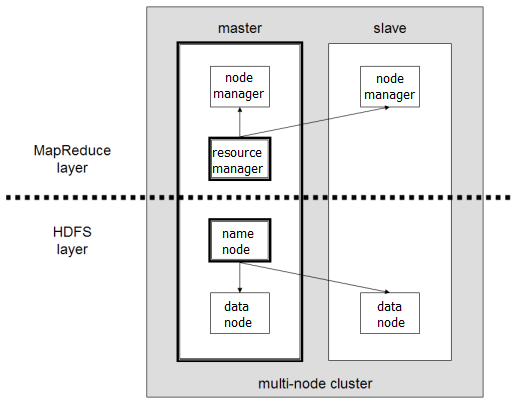
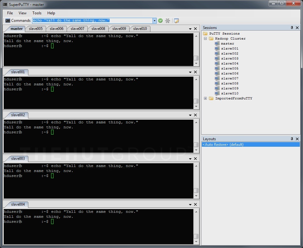
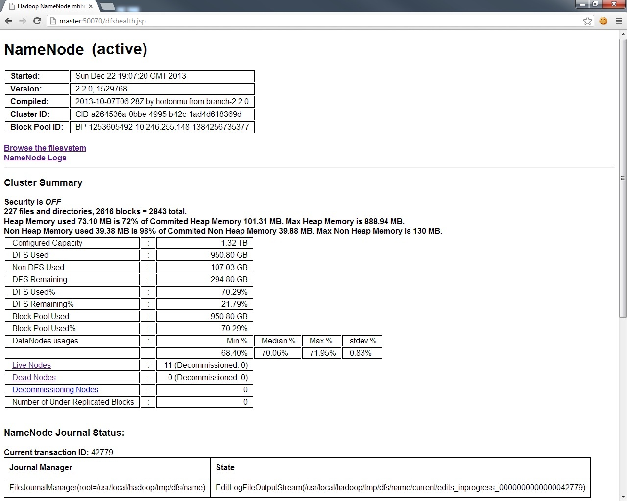
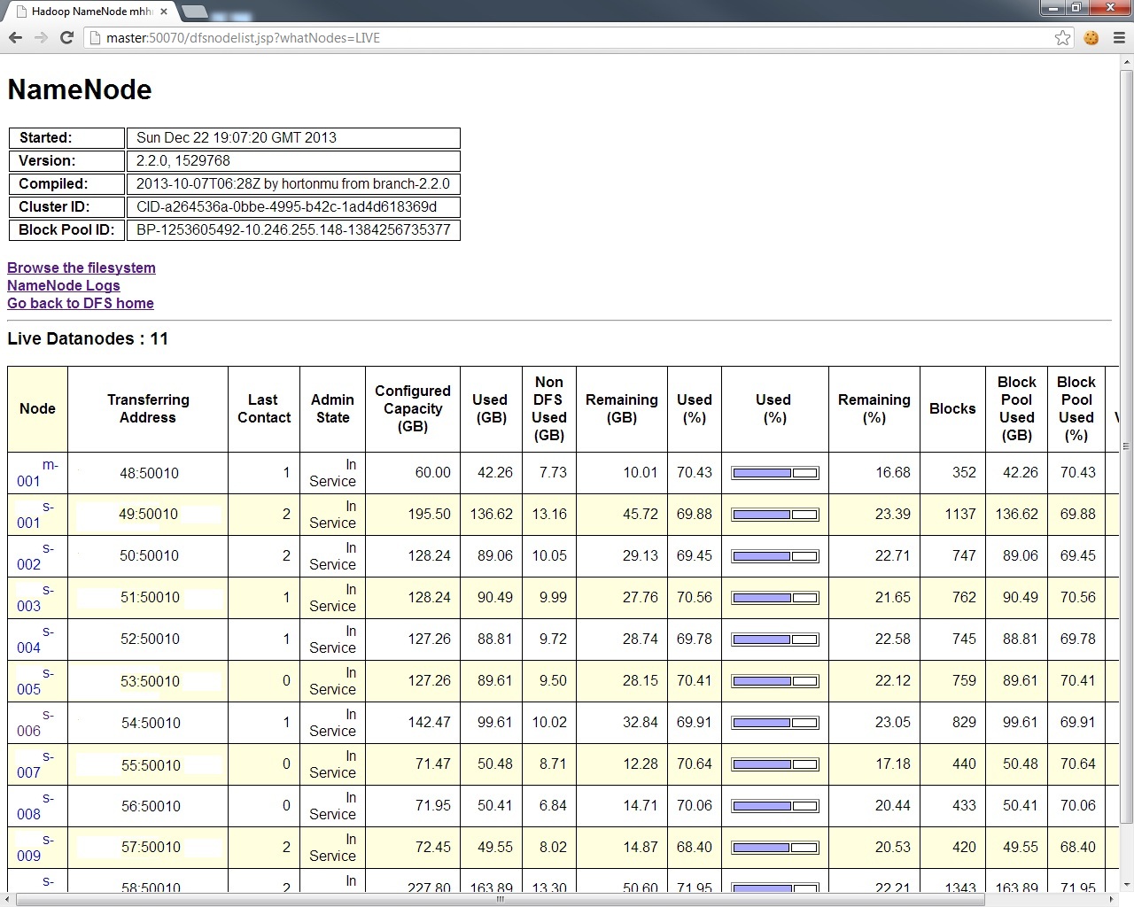
Handling Distributed Search
Elasticsearch is an excellent example of a sophisticated distributed system which hides much of the inherent complexity from the user. Behind the scenes, problems like partitioning documents into shards, balancing shards across the cluster, replicating data to maintain fault-tolerance and efficiently routing requests between nodes are handled. All you have to do is configure a couple of settings in your elasticsearch.yaml – such as the number of shards to split each index into and the number of replicas to keep of each shard.

While configuring distributed search is pretty easy, there are some more complex issues which should be addressed. One of these issues is: how can we make a change to our mapping (i.e. the index) without causing any downtime to our search engine. For an e-commerce company, any form of downtime translates directly to a loss in revenue, and with our large product base, re-populating the search indices is a lengthy process which takes several hours. This problem can be solved using index aliases – an Elasticsearch feature which enables us to set up something similar to a symbolic link – an index alias which always points to a live and fully prepared index. For example, we can set up an alias, products which points to a specific version of our products index:

PUT /products_v1/_alias/products

Now, we can make a change to our mapping and populate a new index, products_v2, wait until we are satisfied that all data has been indexed and shards balanced, before finally switching our alias to point to the new index.

There are some problems that come with the distributed nature of Elasticsearch. Imagine performing a search, getting 10 search results in the response, then refreshing the page and seeing 50 search results. How can search be non-deterministic?! Well, this is a problem that we encountered. This problem comes about as a result of Elasticsearch making optimisations and using approximate term frequencies to determine results. Each shard has a subset of documents in the index, and by default, Elasticsearch will use the shard’s term frequencies as an approximation for the actual term frequencies. When using the common terms query as described earlier, a term may fall under the threshold for being considered a stop word on one shard, but may be over the threshold on another shard. So, depending on which node a query gets routed to, we can end up with different results. Most of the time, this isn’t a problem as term frequencies should be very similar across all shards, providing there is enough data and the data is evenly distributed. But, if it does become a problem, full accuracy can be achieved by changing the default query type to dfs_query_and_fetch, by appending &search_type=dfs_query_then_fetch to the search URI. This query type performs an additional round-trip, collecting term frequencies from all nodes and calculating a global term frequency, before sending the query to all shards and computing results using the global frequencies. This ensures results are always accurate, but comes at the cost of some additional latency.

A similar problem can be seen in faceting. Facet counts are computed on each shard and then aggregated on the node designated as coordinator. If, say, our request is for the top 10 terms within a facet, then each node will return it’s locally computed top 10 facet elements. In cases where there are more than 10 terms, accuracy can be lost. To address this problem, a recent version of Elasticsearch introduced a shard_size attributed which can be set on the facet query, and specifies the number of elements each shard should return. This is separate from the size attribute – i.e. the number of elements we actually want. Asking each shard to return more elements is of course more expensive, but will give higher accuracy when it is needed.

Conclusions

  • It is hard to find a query which works well for every search. If there is a particular search found to yield bad results, it can be easy to optimise towards improving and fixing that search, but then other searches end up suffering as a result. When making changes to the search query, always think: will this work well for both general searches and specific searches?
  • Use filters for faceting, to filter search results without affecting facet counts. Also, Elasticsearch filters are (by default) cached, so can boost performance.
  • The three types of instant search: product suggestions, search suggestions and spelling corrections can be achieved with a single Elasticsearch query – providing the title field is configured with both a shingles and n-grams analyzer.
  • You should always A/B test whenever you make a change to the search experience. It can be invaluable to have good reporting on things like ‘searches which yield no results’ to easily catch problem with changes to the query.
  • Use index aliases to make large changes while maintaining zero-downtime.
  • There can be non-deterministic results with a distributed search engine, but with Elasticsearch these problems can be resolved at the cost of additional latency.
  • The search experience makes a big difference. It not only enables customers to discover the products they are looking for, but a well-tuned search experience can also can help them discover things they weren’t explicitly searching for. We saw significant boosts in revenue from search every time we made improvements to the search engine.

Building a Recommendation Service on AWS with Mahout

Hi all,

Those (two) of my regular readers will know I frequently curse my fool-of-a-took laptop. With this in mind I’ve been meaning to write a tutorial on working with Amazon’s web services for when you don’t have the hardware you need. This isn’t that post but I will assume you’ve already got a cluster to hand with all the bits and bobs you need installed.

If you don’t, don’t worry about it (for now) – I’ll do a post on how to get one of those set up at a later date. For now I’d like to talk about collaborative filtering. This is one of the most prevalent techniques for generating recommendations and with good reason – it’s pretty good. It’s quite a common sense method:

I know that person A likes items 1, 2 and 3 but not item 4.
I know that person B likes item 4 and 3 but not 1 or 2.
I know that person C likes item 1  but not 2, 3 or 4.
I know that person D doesn’t like item 4 – which of the items 1, 2 or 3 should I recommend them?

I’m sure most people reading this will say we should recommend them item 1, then probably item 2 then 3? Certainly item 1 with highest preference. Now if you deconstruct your thought process in coming up with that recommendation I’d wager (not a lot) that it’d be akin to the collaborative filtering algorithm.

Based on the behaviour of people A, B and C we can start to get an idea about which items are rated favourably by the same people versus those that aren’t. User-based collaborative filtering is about finding similar users to person D and looking at what they liked. Item-based collaborative filtering is about finding similar items to the ones person D has rated positively and recommending those.

There are lots of nice articles on collaborative filtering – more often than not when it comes to machine learning I end up recommending Andrew Ng material and this is no exception – check out his machine learning course on Coursera. There’s a whole lecture on collaborative filtering and it’s boss. If my explanation wasn’t enough (if you’re serious about this sort of thing, it shouldn’t be) check out his lectures on the subject and read around on the mathematical details of it all. Make sure you polish up on your linear algebra – you’ll have very large sparse matrices heading your way!

Also, please note that this whole post is just a re-imagining of this post by Amazon: Recommendations using EMR – I liked it and thought I’d give it a go myself with a different data set and technologies I was more familiar with. Now on with the show…

The Data Set

I’m going to be using a publicly available data set containing user ratings of books gathered on Amazon – dataset available here: Book Data Set

There are three files in there – one with all the details of the books, one with all the details of the users and finally one with all the user ratings. Don’t worry about downloading them yet if you’re following this as a tutorial/example – we’ll stick that bit in a script later on.

The Cluster Set-Up

Given that I’m on the free tier and I don’t use AWS at work (we’ve got a nice cluster that handles all our data just fine thank you) I’m a bit ‘over-compute’ happy at the moment and so I’m going to use a 5 node cluster (1 master node and 4 slaves). This isn’t really necessary but then nor is this as a piece of work so I’m not that bothered by practicality at this point. The benefit of using Amazon’s Elastic Mapreduce is that the nodes all come with Hadoop (& Hive/Pig/Mahout/whatever) installed and set up so you don’t have to bother with any of that.

Building a Service

I want to demonstrate how easy it is to turn this sort of thing into a recommendations service (instead of a one-off bit of analysis). Now I’m going to stress that I’m setting this up as an offline batch machine learning method and that there are a few steps I’d change if I were actually setting this up as a real, ‘production’, service.

I’m going to use a Redis database because I’ve got a reasonable amount of memory on these boxes (Redis is an in-memory key-value store), because Redis is really really quick and because I’m used to using Redis with Python. Redis will store the output of my collaborative filtering and I’ll stick a lightweight web framework (Flask) on top of it. This will allow a client to retrieve recommendations for a given user as well as delete them or overwrite them. I’ve decided to add the latter two functions because we don’t live in a perfect world.

I’ll also write a script that’ll update the books, users and ratings files and stick it on a cronjob to run every day. That way, by copying this method you’ll end up with a reasonably scalable, reasonably fast and reasonably up-to-date recommendation service. It’s not the best one out there (heck, it might be the worst) but it goes to show how simple these things are to set up given all the tools that are already written…

The Code

Firstly, we’ll create the cluster using the Elastic Mapreduce CLI:

./elastic-mapreduce --create --alive --name recommendation-service --num-instances 5 --master-instance-type m1.large --slave-instance-type m2.xlarge --ami-version 3.1 --ssh

The --ssh means that once the cluster has been created and all the necessary bits and bobs installed we ssh into the master node

Extracting the data set

 
wget http://www2.informatik.uni-freiburg.de/~cziegler/BX/BX-CSV-Dump.zip
unzip BX-CSV-Dump.zip
sed '1d;' BX-Book-Ratings.csv | tr ';' ',' | tr -d '"' > Book-Ratings.csv}

Unfortunately for us, we’ve got a bit of work to do – the ‘out of the box’ Mahout recommendation algorithm requires user and book ids to be integers and ISBNs are not. To get around this, we use this nifty little script:

#!/usr/bin/python

import sys
import re

isbn_dictionary = {}

counter = 0

with open('Book-Ratings.csv', 'rb') as f:
    with open('New-Book-Ratings.csv', 'w') as g:
        with open('Book-Mappings.csv', 'w') as h:
            for line in f:
                try:
                    user, book, rating = line.split(',')
                except:
                    continue
                try:
                    index = isbn_dictionary[book]
                except:
                    isbn_dictionary[book] = counter
                    index = counter
                    h.write("%s,%dn" % (book, counter))
                    counter += 1
                g.write("%d,%d,%dn" % (int(user), index, int(rating)))

Now we’ve got data in the format our Mahout recommender is expecting let’s put it in HDFS and run our algorithm

hadoop fs -put New-Book-Ratings.csv /New-Book-Ratings.csv
mahout recommenditembased --input /New-Book-Ratings.csv --output recommendations --numRecommendations 10 --similarityClassname SIMILARITY_COSINE

Now we play the waiting game…
Actually, while that’s running, open up another SSH session to that terminal and run these commands

sudo easy_install redis flask
wget http://download.redis.io/releases/redis-2.8.13.tar.gz
tar xzf redis-2.8.13.tar.gz
cd redis-2.8.13
make
./src/redis-server &
cd

Now Redis is installed and running and we’ve got the necessary Python libraries we can create the following server…

import redis
import os

isbn_dictionary = {}

with open('Book-Mappings.csv', 'rb') as f:
    for line in f:
        isbn, counter = line.split(',')
        isbn_dictionary[int(counter)] = isbn

r = redis.StrictRedis(host='localhost', port=6379, db=0)

p = os.popen('hadoop fs -cat recommendations/part*')

for recommendation in p:
    user, recommendations = recommendation.split('t')
    recommendations = [entry.split(':')[0] for entry in recommendations.replace('[', '').replace(']','').split(',')]
    recommendations = [isbn_dictionary[int(entry)] for entry in recommendations]
    r.set(int(user), recommendations)

Now we’ve populated our database with all the recommendations we generated with our Mahout job. Now we’ll set something up (called webserver.py) to return these items to a client (as well as allow modifications to be made).

import redis
from flask import Flask
r = redis.StrictRedis(host='localhost', port=6379, db=0)

app = Flask(__name__)

@app.route('/user/<user_id>', methods = ['GET', 'POST', 'PUT', 'DELETE'])
def restful_api(user_id):
    if request.method == 'GET':
        recommendations = r.get(int(user_id))
        return recommendations if recommendations else "User %d does not exist" % int(user_id)
    elif request.method == 'POST':
        if request.headers['Content-Type'] == 'application/json':
            r.set(int(user_id), request.json)
            return "Successfully set recommendations for user %d" % int(user_id)
        else:
            return False
    elif request.method == 'DELETE':
        if r.exists(int(user_id)):
            r.delete(int(user_id))
            return "Successfully deleted recommendations for user %d" % int(user_id)
        else:
            return "User %d does not exist" % int(user_id)
    elif request.method == 'PUT':
        if request.headers['Content-Type'] == 'application/json':
            r.set(int(user_id), request.json)
            return "Successfully set recommendations for user %d" % int(user_id)
        else:
            return "Require JSON put"
    else:
        return "No idea what you've done here, but don't do it again"

if __name__ == '__main__':
    app.run()

Now we’ve built our client-facing recommendations service let’s ‘deploy’ it and give it a test

python webserver.py &
curl -X GET localhost:5000/user/277965
curl -X DELETE localhost:5000/user/277965
curl -X GET localhost:5000/user/277965

Summary

We’ve not done anything that tricky but in a fairly short time we’ve managed to build something that’d be at least part way useful to a small business somewhere looking for recommendations for their users. It’s not a great leap from this and a genuine production ready system – you don’t need 5 Hadoop nodes running all the time for a 20 minute Mahout job and I’m uncomfortable using Flask and local files for a serious system. As such, you’d likely put together a couple of nodes, each with their own copy of the recommendations set in memory. One of them would create a cluster, get any new data a generate the data set as often as you saw fit – communicating it to the other node. Finally, you’d add a few more actions to the server and make sure it could be called by whichever clients need it (and block everybody else).

As I say, nothing earth-shattering but a solid base on which to build a recommendations system.

I am become death.


Installing Hadoop 2.4 on Ubuntu 14.04

Hey all,

Another of my ‘getting my new operating system set up with all the bits of kit I use’ – this time we’ll be on Hadoop (and HDFS). There’s a very strong chance that this post will end up a lot like Sean’s post – Hadoop from spare-change. If there are any differences it’ll be for these reasons three:
1.) He was using Ubuntu Server 13.04 not Ubuntu Desktop 14.04
2.) He was using Hadoop 2.2 not Hadoop 2.4
3.) He was setting up a whole bunch of nodes – I’m stuck with this oft-abused laptop

Anywho – on with the show.

Step 1:

Download Hadoop from Apache: I’ll be using this mirror but I trust that if you’re not in England, you can likely find a more suitable one:
http://mirror.ox.ac.uk/sites/rsync.apache.org/hadoop/common/hadoop-2.4.0/hadoop-2.4.0.tar.gz

If you’re trying to stick to the terminal/don’t have a GUI then go with this:

wget http://mirror.ox.ac.uk/sites/rsync.apache.org/hadoop/common/hadoop-2.4.0/hadoop-2.4.0.tar.gz

Find your way to wherever you downloaded the tar.gz file and untar it using the following command:

tar -xzf hadoop-2.4.0.tar.gz

Sorry if I’m teaching you to suck eggs – everybody has to start somewhere right?

Has it worked up till here?

Run the following command in the same directory you ran the above tar command:

ls | grep hadoop | grep -v *.gz

If there’s at least one line returned (ideally hadoop-2.4.0) then you’re good up till here.

Step 2:

Let’s move everything into a more appropriate directory:

sudo mv hadoop-2.4.0/ /usr/local
cd /usr/local
sudo ln -s hadoop-2.4.0/ hadoop

We create that link to allow us to write scripts/programs that interact with Hadoop that won’t need changing if we upgrade our Hadoop version. All we’ll do is install the new version and point the Hadoop folder to the new version instead. Ace.

Has it worked up to here?

Run this command anywhere:

whereis hadoop

If the output is:
hadoop: /usr/local/hadoop
you may proceed.

Step 3:

Righty, now we’ll be setting up a new user and permissions and all that guff. I’ll steal directly from Michael Noll’s tutorial here and go with:

sudo addgroup hadoop
sudo adduser --ingroup hadoop hduser
sudo adduser hduser sudo
sudo chown -R hduser:hadoop /usr/local/hadoop/

Has it worked up to here?

Type:

ls -l /home/ | grep hadoop

If you see a line then you’re in the money.

Step 4:

SSH is a biggy – possibly not so much for the single node tutorial but when we were setting up our first cluster, SSH problems probably accounted for about 90% of all head-scratching with the remaining 10% being nits.


su - hduser
sudo apt-get install ssh
ssh-keygen -t rsa -P ""
cat ~/.ssh/id_rsa.pub >> ~/.ssh/authorized_keys

So we switch to our newly created user, generate an SSH key and get it added to our authorized keys. Unfortunately, Hadoop and ipv6 don’t play nice so we’ll have to disable it – to do this you’ll need to open up /etc/sysctl.conf and add the following lines to the end:


net.ipv6.conf.all.disable_ipv6 = 1
net.ipv6.conf.default.disable_ipv6 = 1
net.ipv6.conf.lo.disable_ipv6 = 1

Fair warning – you’ll need sudo privileges to modify the file so might want to open up your file editor like this:

sudo apt-get install gksu
gksu gedit /etc/sysctl.conf

If you’re set on using terminal then this’ll do it:

echo "net.ipv6.conf.all.disable_ipv6 = 1" | sudo tee -a /etc/sysctl.conf
echo "net.ipv6.conf.default.disable_ipv6 = 1" | sudo tee -a /etc/sysctl.conf
echo "net.ipv6.conf.lo.disable_ipv6 = 1" | sudo tee -a /etc/sysctl.conf

Rumour has it that at this point you can run
sudo service networking restart
and kapeesh – ipv6 is gone. However, Atheros and Ubuntu seem to have a strange sort of ‘not working’ thing going on and so that command doesn’t work with my wireless driver. If the restart fails, just restart the computer and you should be good.

(if you’re terminal only : sudo shutdown -r now )

Has it worked up to here?

If you’re stout of heart, attempt the following:

su - hduser
ssh localhost

If that’s worked you be greeted with a message along the lines of ‘Are you sure you want to continue connecting?’ The answer you’re looking for at this point is ‘yes’.

If it hasn’t worked at this point run the following command:
cat /proc/sys/net/ipv6/conf/all/disable_ipv6

If the value returned is 0 then you’ve still not got ipv6 disabled – have a re-read of that section and see if you’ve missed anything.

Step 5:
I’m going to assume a clean install of Ubuntu on your machine (because that’s what I’ve got) – if this isn’t the case, it’s entirely likely you’ll already have Java installed. If so, find your JAVA_HOME (lots of tutorials on this online) and use that for the upcoming instructions. I’m going to be installing Java from scratch:

sudo apt-get update
sudo apt-get install default-jdk

Given a bit of luck, you’ll now have Java on your computer (I do on mine) and you’ll be able to set your environment variables. Open up your bashrc file:

su - hduser
gksu gedit .bashrc

and add the following lines:

export HADOOP_HOME=/usr/local/hadoop
export JAVA_HOME=/usr

and follow up with this command:
source ~/.bashrc

If you’ve deviated from any of the instructions above, those lines are likely to be different. You can find what your java home should be by running the following command:
which java | sed -e 's/(.*)/bin/java/1/g'

Your Hadoop home will be wherever you put it in step 2.

Has it worked up to here?

So many different ways to test – let’s run our first Hadoop command:

/usr/local/hadoop/bin/hadoop version

If that worked with no error (and gave you your Hadoop version) then you’re laughing.

Step 6:

Configuration of Hadoop (and associated bits and bobs) – we’re going to be editing a bunch of files so pick your favourite file editor and get to work. First things first though, you’re going to want some place for HDFS to save your files. If you’ve going to be storing anything big/bought external storage for this purpose now is the time to deviate from this tutorial. Otherwise, this should do it:


su - hduser
mkdir /usr/local/hadoop/data

Now for the file editing:

(only necessary when running a multi-node cluster, but let’s do it in case we ever get more nodes to add)
1.) /usr/local/hadoop/etc/hadoop/hadoop-env.sh
Change export JAVA_HOME=${JAVA_HOME} to match the JAVA_HOME you set in your bashrc (for us JAVA_HOME=/usr).
Also, change this line:
export HADOOP_OPTS="$HADOOP_OPTS -Djava.net.preferIPv4Stack=true
to be

export HADOOP_OPTS="$HADOOP_OPTS -Djava.net.preferIPv4Stack=true -Djava.library.path=$HADOOP_PREFIX/lib"

And finally, add the following line:
export HADOOP_COMMON_LIB_NATIVE_DIR=${HADOOP_PREFIX}/lib/native

2.) /usr/local/hadoop/etc/hadoop/yarn-env.sh
Add the following lines:

export HADOOP_CONF_LIB_NATIVE_DIR=${HADOOP_PREFIX:-"/lib/native"}
export HADOOP_OPTS="-Djava.library.path=$HADOOP_PREFIX/lib"

3.) /usr/local/hadoop/etc/hadoop/core-site.xml
Change the whole file so it looks like this:

<?xml version="1.0" encoding="UTF-8"?>
<?xml-stylesheet type="text/xsl" href="configuration.xsl"?>
<configuration>
<property>
  <name>fs.default.name</name>
  <value>hdfs://localhost:9000</value>
</property>
<property>
  <name>hadoop.tmp.dir</name>
  <value>/usr/local/hadoop/data</value>
</property>
</configuration>

4.) /usr/local/hadoop/etc/hadoop/mapred-site.xml
Change the whole file so it looks like this:

<?xml version="1.0"?>
<?xml-stylesheet type="text/xsl" href="configuration.xsl"?>

<configuration>
    <property>
        <name>mapreduce.framework.name</name>
        <value>yarn</value>
    </property>
</configuration>

5.) /usr/local/hadoop/etc/hadoop/hdfs-site.xml
Change the whole file so it looks like this:

<?xml version="1.0" encoding="UTF-8"?>
<?xml-stylesheet type="text/xsl" href="configuration.xsl"?>

<configuration>
    <property>
        <name>dfs.replication</name>
        <value>3</value>
    </property>
</configuration>

6.) /usr/local/hadoop/etc/hadoop/yarn-site.xml
Change the whole file so it looks like this:

<?xml version="1.0"?>
<configuration>
    <property>
        <name>yarn.nodemanager.aux-services</name>
        <value>mapreduce_shuffle</value>
    </property>
    <property>
        <name>yarn.nodemanager.aux-services.mapreduce_shuffle.class</name>
        <value>org.apache.hadoop.mapred.ShuffleHandler</value>
    </property>
    <property>
        <name>yarn.resourcemanager.resource-tracker.address</name>
        <value>localhost:8025</value>
    </property>
    <property>
        <name>yarn.resourcemanager.scheduler.address</name>
        <value>localhost:8030</value>
    </property>
    <property>
        <name>yarn.resourcemanager.address</name>
        <value>localhost:8050</value>
    </property>
</configuration>

Annnd we’re done 🙂 Sorry about that – if I could guarantee that you’d be using the same file paths and OS as me then I’d let you wget those files from a Github somewhere but alas, I think that’s likely to cause more headaches than it solves. Don’t worry, we’re nearly there now 🙂

Has it worked up to here?

Run the following command:

/usr/local/hadoop/bin/hadoop namenode -format

If that works, you’re 20% of the way there.

Then, run:

/usr/local/hadoop/sbin/start-dfs.sh

If that seems to work without throwing up a bunch of errors:

/usr/local/hadoop/sbin/start-yarn.sh

If that’s worked, you can safely say you’ve got Hadoop running on your computer 🙂 Get it on the LinkedIn as a strength as soon as possible 😉

Conclusion
Now you’ve got Hadoop up and running on your computer, what can you do? Well, unfortunately with that single node and single hard disk, not much you couldn’t have done without it. However, if you’re just getting started with Linux and Hadoop you’ll have hopefully learnt a bit on the way to setting up your cluster.

Hadoop From Spare Change

A Data Scientist happened upon a load of stuff – junk, at first glance – and wondered, as was his wont, “what can I get out of this?”

Conceded: as an opening line this is less suited to a tech blog than an old-fashioned yarn. In an (arguably) funny way, this isn’t far from the truth. My answer: get some holism down your neck. Make it into a modest, non-production Hadoop cluster and enjoy a large amount of fault-tolerant storage, faster processing of large files than you’d get on a single high-spec machine, the safety of not having placed all your data-eggs in one basket, and an interesting challenge. Squeeze the final, and not inconsiderable, bit of business value out of it.

To explain, when I say “stuff”, what I mean is 6 reasonable but no longer DC-standard rack servers, and more discarded dev desktops than you can shake a duster at. News of the former reached my Data Scientist colleague and I by way of a last call before they went into the skip; I found the latter buried in the boiler room when looking for bonus cabling. As a northerner with a correspondingly traumatic upbringing, instinct won out and, being unable to see it thrown away, I requested to use the hardware.

I’m not gonna lie. They were literally dumped at my feet, “unsupported”. Fortunately, the same qualities of character that refused to see the computers go to waste saw me through the backbreaking physical labour of racking and cabling them up. Having installed Ubuntu Server 13 on each of the boxes, I had soon pinged my desktop upstairs successfully and could flee the freezing server room to administrate from upstairs. Things picked up from here, generally speaking.

The hurdle immediately ahead was the formality of installing and correctly configuring Hadoop on all of the boxes, and this, you may be glad to know, brings me to the point of this blog post. Those making their first tentative steps into the world of Hadoop may be interested to know how exactly this was achieved, and indeed, I defy anyone to point me towards a comprehensive Hadoop-from-scratch quick start which leaves you with a working version of a recent release of Hadoop. Were it not for the fact that Hadoop 2.x has significant configuration differences to Hadoop 1.x, Michael Noll’s excellently put-together page would be ideal. It’s still a superb pointer in itself and was valuable to me during my first youthful fumblings with Hadoop 18 months ago. The inclusion of important lines of bash neatly quashes the sorts of ambiguity that may arise from instructions like “move the file to HDFS” which you sometimes find.

In any case, motivated by the keenness to see cool technology adopted as easily and widely as possible, I propose in this to briefly explain the configuration steps necessary to get me into a state of reverse cartography. (Acknowledged irony: there will probably be a time when someone reads this and it’s out of date. Apologies in advance.) Having set up a single node, it’s actually more of a hassle to backtrack over your configuration to add more nodes than to just go straight to a multi-node cluster. Here’s now to do the latter.

Setting the Scene

The Hadoop architecture can be summarised in saying that it elegantly facilitates doing two things in a distributed manner: storing files, and processing files. The two poles of the Hadoop world which respectively deal with these are known as the DFS (distributed file system) layer, and the MapReduce layer. Each layer knows about the other, but can, and indeed must, be configured, administrated and used fairly independently across a cluster. There’s an interesting history to both of these computing paradigms, and many papers written by the likes of Google and Facebook describing their inner workings. A quick Youtube yields some equally illuminating talks. My personal favourites on the two layers are this for HDFS and this for MapReduce.

Typically a cluster of computers (nodes) will have 1 master node, which coordinates the distribution of storage and processing, and (n-1) slave nodes which do the actual stuff. The modules (daemons) in Hadoop 2.x which control all of these are as below.

Master Slaves
DFS  Namenode  Datanode
MR  Resourcemanager  Nodemanager

Obligatory diagram:

Hadoop Architecture
Illuminating.

Based on your current cluster setup, Hadoop makes a bunch of intelligent decisions about where to put files, and which machines to do certain bits of processing on, motivated by maximising redundancy and fault tolerance by clever replication choices, minimising network overhead, optimally leveraging each bit of hardware, and so on. The way that the architecture makes these decisions in such a way that you, the Hadoop developer, don’t have to worry about them, is where the real beauty and power of Hadoop lies. We’ll see later in this blog how, whilst HDFS and MapReduce are breathtakingly complex and scalable under the bonnet, leveraging their power is no more difficult than performing normal straightforward file system operations and file processing in Linux.

So. At this stage, all you have is a collection of virginal, disparate machines that can see each other on the network, but beyond that share no particular sense of togetherness. Each must undergo the same setup procedure before it’s ready to pull its weight in the cluster. In a production environment, this would be achieved by means of an automated deployment script, so that nodes could be added easily and arbitrarily, but that is both overkill and an unnecessary complication here. Good old-fasioned Bash elbow grease will see us through.

Having said that, one expedient whose virtues I will extol is a little gem of software called SuperPutty, which will send the same command from any single Windows PC to all the Linux boxes simultaneously, in so doing greatly reducing repetitiveness and cutting out chances for human error:

SuperPutty
Using SuperPutty to send commands en-masse is only the same as doing the same thing on each box in sequence.

Connect to all the boxes and make sure you’re at the same bash prompt on all of them. SuperPutty will let you store connection authentication details to save you even more time in swiftly connecting to every  machine in your cluster. (Disclaimer: if you do store passwords, anyone with Linux knowledge who finds your unattended, unlocked PC could connect to your cluster and perform wild-rogue Hadoop operations on your data. Think carefully.)

Masters and Slaves

One of your computers will be the master node, and the rest slaves. The master’s disks are the only ones that need to have an appropriate RAID configuration, since Hadoop itself handles replication in a better way in HDFS: choose JBOD for the slaves. If one of your machines stands above the rest in terms of RAM and/or processing power, choose this as the master.

Since Hadoop juggles data around amongst nodes like there’s no tomorrow, there are a few networking prerequisites to sort, to make sure it can do this unimpeded and all nodes can communicate freely with each other.

Hosts

Working with IPs is a lot like teaching cats to read: it quickly becomes tedious. The file /etc/hosts enables you to specify names for IP addresses, then you can just use the names. Every node needs to know about every other node. You’ll want your hosts file on each of the boxes to look something like this so you can refer to (eg) slave 11 without having to know (or calculate!) slave 11’s IP:
123.1.1.25 master
123.1.1.26 slave001
123.1.1.27 slave002
123.1.1.28 slave003
123.1.1.29 slave004
... etc

It’s also a good idea to disable IPv6 on the Hadoop boxes to avoid potential confusion regarding localhost addresses… Fire every box the below commands to append the necessary lines to /etc/sysctl.conf…
sean@node:~$ echo "#disable ipv6" | sudo tee -a /etc/sysctl.conf
sean@node:~$ echo "net.ipv6.conf.all.disable_ipv6 = 1" | sudo tee -a /etc/sysctl.conf
sean@node:~$ echo "net.ipv6.conf.default.disable_ipv6 = 1" | sudo tee -a /etc/sysctl.conf
sean@node:~$ echo "net.ipv6.conf.lo.disable_ipv6 = 1" | sudo tee -a /etc/sysctl.conf

The machines need to be rebooted for the changes to come into effect…
sean@node:~$ sudo shutdown -r now

Once they come back up, run the following to check whether IPv6 has indeed been disabled. A value of 1 would indicate that all is well.
sean@node:~$ cat /proc/sys/net/ipv6/conf/all/disable_ipv6

Setting up the Hadoop User

For uniformity across your cluster, you’ll want to have a dedicated Hadoop user with which to connect and do work…
sean@node:~$ sudo addgroup hadoop
sean@node:~$ sudo adduser --ingroup hadoop hduser
sean@node:~$ sudo adduser hduser sudo

We’ll now switch users and work as the new Hadoop user…
sean@node:~$ su - hduser
hduser@node:~$

SSH Promiscuity

Communication between nodes take place by way of the secure shell (SSH) protocol. The idea is to enable every box to passwordlessly use an SSH connection to itself, and then copy those authentication details to every other box in the cluster, so that any given box is on familiar terms with any other and Hadoop is unshackled to work its magic!

Firstly, send every box the instruction to make a passwordless SSH key to itself for hduser:
hduser@node:~$ ssh-keygen -t rsa -P ""

Bash will prompt you for a location in which to store this newly-created key. Just press enter for default:
Generating public/private rsa key pair.
Enter file in which to save the key (/home/hduser/.ssh/id_rsa): Created directory '/home/hduser/.ssh'.
Your identification has been saved in /home/hduser/.ssh/id_rsa.
Your public key has been saved in /home/hduser/.ssh/id_rsa.pub
The key fingerprint is: 9b:82...................:0e:d2 hduser@ubuntu
The key's randomart image is: [weird ascii image]

Copy this new key into the local list of authorised keys:
hduser@node:~$ cat $HOME/.ssh/id_rsa.pub >> $HOME/.ssh/authorized_keys

The final step in enabling local SSH is to connect – this will save the fingerprint of the host to the list of familiar hosts.
hduser@node:~$ ssh hduser@localhost
The authenticity of host 'localhost (::1)' can't be established.
RSA key fingerprint is d7:87...............:36:26
Are you sure you want to continue connecting? yes
Warning: permanently added 'localhost' (RSA) to the list of known hosts.

Now, to allow all the boxes to enjoy the same level of familiarity with each other, fire them all this command:
hduser@node:~$ ssh-copy-id -i $HOME/.ssh/id_rsa.pub hduser@master

This will make every box send its SSH key to the master node. Unfortunately, you have to repeat this to tell every box to send its key to every node…
hduser@node:~$ ssh-copy-id -i $HOME/.ssh/id_rsa.pub hduser@slave001
hduser@node:~$ ssh-copy-id -i $HOME/.ssh/id_rsa.pub hduser@slave002
hduser@node:~$ ssh-copy-id -i $HOME/.ssh/id_rsa.pub hduser@slave003
etc...

Finally, and this is also a bit tedious, via SuperPutty make every box SSH to each box in turn and check that all’s well. Ie, send them all:
hduser@node:~$ ssh master

…check that they all have…
hduser@node:~$ ssh slave001

… check that they all have… etc.

This is a one-time thing; after any box has connected to any other one time, the link between them remains.

Java

The next prerequisite to sort is a Java environment, as the Hadoop core is written Java (although you can harness the power of MapReduce in any language you please, as we shall see). If you’re fortunate, your machines will have internet access, in which case fire the following command to them all using SuperPutty:
hduser@node:~$ sudo apt-get install openjdk-6-jre
If like mine, however, your machines were considered ticking chemical time bombs by infrastructure and hence weren’t granted internet access, what you’ll want to do is download a JDK to a computer that does have internet access and can also see your Hadoop boxes on the network, and fire the files over from there. So on your internet-connected box:
32 bit version:
hduser@node:~$ wget --no-cookies --no-check-certificate --header "Cookie: gpw_e24=http://www.oracle.com/" http://download.oracle.com/otn-pub/java/jdk/6u34-b04/jre-6u34-linux-i586.bin

64 bit version:
hduser@node:~$ wget --no-cookies --no-check-certificate --header "Cookie: gpw_e24=http://www.oracle.com/" http://download.oracle.com/otn-pub/java/jdk/6u45-b06/jdk-6u45-linux-x64.bin

Now then! Each of your Hadoop nodes wants to connect to this box and pull over the Java files. Find its IP by typing ifconfig, and then fire this command to all of your Hadoop nodes:
hduser@node:~$ scp user@internetbox:/locationoffile/rightarchtecturefile.bin $HOME

Be careful to get the edition matching the machine, be it 32bit or 64bit.

Now execute the following on the Hadoop machines to install Java…

32 bit machines:
hduser@node:~$ chmod u+x jre-6u34-linux-i586.bin
hduser@node:~$ ./jre-6u34-linux-i586.bin
hduser@node:~$ sudo mkdir -p /usr/lib/jvm
hduser@node:~$ sudo mv jre1.6.0_34 /usr/lib/jvm/
hduser@node:~$ sudo update-alternatives --install "/usr/bin/java" "java" "/usr/lib/jvm/jre1.6.0_34/bin/java" 1
hduser@node:~$ sudo update-alternatives --install "/usr/lib/mozilla/plugins/libjavaplugin.so" "mozilla-javaplugin.so" "/usr/lib/jvm/jre1.6.0_34/lib/i386/libnpjp2.so" 1
hduser@node:~$ sudo update-alternatives --install "/usr/bin/javaws" "javaws" "/usr/lib/jvm/jre1.6.0_34/bin/javaws" 1
hduser@node:~$ sudo update-alternatives --config java
hduser@node:~$ sudo update-alternatives --config javac
hduser@node:~$ export JAVA_HOME=/usr/lib/jvm/jre1.6.0_34/

64 bit machines:
hduser@node:~$ chmod u+x jdk-6u45-linux-x64.bin
hduser@node:~$ ./jdk-6u45-linux-x64.bin
hduser@node:~$ sudo mv jdk1.6.0_45 /opt
hduser@node:~$ sudo update-alternatives --install "/usr/bin/java" "java" "/opt/jdk1.6.0_45/bin/java" 1
hduser@node:~$ sudo update-alternatives --install "/usr/bin/javac" "javac" "/opt/jdk1.6.0_45/bin/javac" 1
hduser@node:~$ sudo update-alternatives --install "/usr/lib/mozilla/plugins/libjavaplugin.so" "mozilla-javaplugin.so" "/opt/jdk1.6.0_45/jre/lib/amd64/libnpjp2.so" 1
hduser@node:~$ sudo update-alternatives --install "/usr/bin/javaws" "javaws" "/opt/jdk1.6.0_45/bin/javaws" 1
hduser@node:~$ sudo update-alternatives --config java
hduser@node:~$ sudo update-alternatives --config javac
hduser@node:~$ export JAVA_HOME=/opt/jdk1.6.0_45/

Finally, test by firing all machines
hduser@node:~$ java --version

You should see something like this:
hduser@node:~$ java -version
java version "1.6.0_45"
Java(TM) SE Runtime Environment (build 1.6.0_45-b06)
Java HotSpot(TM) 64-Bit Server VM (build 20.45-b01, mixed mode)

Installing Hadoop

Download Hadoop 2.2.0 into the directory /usr/local from the best possible source:
hduser@node:~$ cd /usr/local
hduser@node:~$ wget http://mirror.ox.ac.uk/sites/rsync.apache.org/hadoop/core/hadoop-2.2.0/hadoop-2.2.0.tar.gz

If your boxes don’t have internet connectivity, use the same workaround we used above to circuitously get Java.

Unzip, tidy up and make appropriate ownership changes:
hduser@node:~$ sudo tar xzf hadoop-2.2.0.tar.gz
hduser@node:~$ sudo mv hadoop-2.2.0 hadoop
hduser@node:~$ sudo chown -R hduser:hadoop hadoop

Finally, append the appropriate environment variable settings and aliases to the bash configuration file:
hduser@node:~$ echo "" | sudo tee -a $HOME/.bashrc
hduser@node:~$ echo "export HADOOP_HOME=/usr/local/hadoop" | sudo tee -a $HOME/.bashrc
hduser@node:~$ echo "" | sudo tee -a $HOME/.bashrc

#32 bit version:
hduser@node:~$ echo "export JAVA_HOME=/usr/lib/jvm/jre1.6.0_34" | sudo tee -a $HOME/.bashrc

#64 bit version:
hduser@node:~$ echo "export JAVA_HOME=/opt/jdk1.6.0_45" | sudo tee -a $HOME/.bashrc

hduser@node:~$ echo "" | sudo tee -a $HOME/.bashrc
hduser@node:~$ echo "unalias fs &> /dev/null" | sudo tee -a $HOME/.bashrc
hduser@node:~$ echo "alias fs &>"hadoop fs"" | sudo tee -a $HOME/.bashrc
hduser@node:~$ echo "unalias hls &> /dev/null" | sudo tee -a $HOME/.bashrc
hduser@node:~$ echo "alias hls="fs -ls" | sudo tee -a $HOME/.bashrc
hduser@node:~$ echo "" | sudo tee -a $HOME/.bashrc
hduser@node:~$ echo "export PATH=$PATH:$HADOOP_HOME/bin" | sudo tee -a $HOME/.bashrc

There are a few changes that must be made to the configuration files in /usr/local/hadoop/etc/hadoop which inform the HDFS and MapReduce layers. Editing these on every machine at once via SuperPutty requires skill, especially when, having made the changes, you realise that you can’t send an “escape” character to every machine at once. There’s a solution involving mapping other, sendable, characters to the escape key, but that’s “out of scope” here 😉 Here’s what the files should look like.

core-site.xml

It needs to look like this on all machines, master and slave alike:

[code language=”xml”]
<configuration>
<property>
<name>fs.default.name</name>
<value>hdfs://master:9000</value>
</property>
<property>
<name>hadoop.tmp.dir</name>
<value>/usr/local/hadoop/tmp</value>
</property>
</configuration>[/code]

hadoop-env.sh

There’s only one change that needs to be made to this mofo; locate the line which specifies JAVA_HOME (helpfully commented with “the Java implementation to use”). Assuming a Java setup like that described above, this should read

32 bit machines:

export JAVA_HOME=/usr/lib/jvm/jre1.6.0_34/

64 bit machines:
export JAVA_HOME=/opt/jdk1.6.0_45/

hdfs-site.xml

This specifies the replication level of file blocks. Note that your physical storage size will be divided by this number to give the storage you’ll have in HDFS.

[code language=”xml”]
<configuration>
<property>
<name>dfs.replication</name>
<value>3</value>
</property>
</configuration>[/code]

Additionally, it’s necessary to create a local directory on each box for Hadoop to use:
hduser@node:~$ sudo mkdir -p /app/hadoop/tmp
hduser@node:~$ sudo chown hduser:hadoop /app/hadoop/tmp

mapred-site.xml

Which MapReduce implementation to use. At the moment we’re on YARN (“Yet Another Resource Negotiator”…………).

[code language=”xml”]
<configuration>
<property>
<name>mapreduce.framework.name</name>
<value>yarn</value>
</property>
</configuration>[/code]

yarn-site.xml

Controls the actual MapReduce configuration. Without further ado, this is what you want:

[code language=”xml”]
<configuration>
<property>
<name>yarn.nodemanager.aux-services</name>
<value>mapreduce_shuffle</value>
</property>
<property>
<name>yarn.nodemanager.aux-services.mapreduce_shuffle.class</name>
<value>org.apache.hadoop.mapred.ShuffleHandler</value>
</property>
<property>
<name>yarn.resourcemanager.resource-tracker.address</name>
<value>master:8025</value>
</property>
<property>
<name>yarn.resourcemanager.scheduler.address</name>
<value>master:8030</value>
</property>
<property>
<name>yarn.resourcemanager.address</name>
<value>master:8040</value>
</property>
</configuration>[/code]

Slaves

In short, the master needs to consider itself and every other node a slave. Each slave needs to consider itself, and itself only, a slave. The entirety of your slaves file ought to look like this:

Master:
master
slave001
slave002
slave003
etc

Slave xyz:
slavexyz

Formatting the Filesystem

Much like manually deleting your data, formatting a HDFS filesystem containing data will delete any data you might have in it, so don’t do that if you don’t want to delete your data. Warnings notwithstanding, execute the following on the master node to format the HDFS namespace:
hduser@master:~$ cd /usr/local/hadoop
hduser@master:~$ bin/hadoop namenode -format

Bringing up the Cluster

This is the moment that the band strikes up. If you’re not already there, switch to the Hadoop directory…
hduser@master:~$ cd /usr/local/hadoop

Fire this shizz to start the DFS layer:
hduser@master:/usr/bin/hadoop$ sbin/start-dfs.sh

You should see this kind of thing:
WARN util.NativeCodeLoader: Unable to load native-hadoop library for your platform... using builtin-java classes where applicable
starting namenodes on [master]
master: starting namenode, logging to /usr/local/hadoop/logs/hadoop-hduser-namenode-master.out
slave001: starting datanode, logging to /usr/local/hadoop/logs/hadoop-hduser-datanode-slave001.out
slave002: starting datanode, logging to /usr/local/hadoop/logs/hadoop-hduser-datanode-slave002.out
slave003: starting datanode, logging to /usr/local/hadoop/logs/hadoop-hduser-datanode-slave003.out
...etc

Now start the MapReduce layer:
hduser@master:/usr/local/hadoop$ sbin/start-yarn.sh

Expect to be greeted by something like this:
starting yarn daemons
starting resourcemanager, logging to /usr/local/hadoop/logs/yarn-hduser-resourcemanager-master.out
slave001: starting nodemanager, logging to /usr/local/hadoop/logs/yarn-hduser-nodemanager-slave001.out
slave002: starting nodemanager, logging to /usr/local/hadoop/logs/yarn-hduser-nodemanager-slave002.out
slave003: starting nodemanager, logging to /usr/local/hadoop/logs/yarn-hduser/nodemanager-slave003.out
...

Also start the job history server…
hduser@master:/usr/local/hadoop$ sbin/mr-jobhistory-daemon.sh start historyserver

Surveying One’s Empire

By this stage your Hadoop cluster is humming like a dynamo. There are several web interfaces which provide a tangible window into the specification of the cluster as a whole…

For the DFS layer, have a look at http://master:50070.

DFS Interface

And for a breakdown of the exact condition of each node in your DFS layer,

DFS Interface 2

And for the MapReduce layer, look at http://master:8088,

YARN Interface

The First Distributed MapReduce

MapReduce is nothing more than a certain way to phrase a script to process a file, which is friendly to distributed computing. There’s a mapper, and a reducer. The “mapper” must be able to process any arbitrary fragment of the file (eg, count the number of occurrences of something within that fragment), independently and obliviously of the contents of the rest of the file. This is why it’s so scalable. The “reducer” aggregates the outputs of the mappers to give the final result (eg, sum up the occurrences of something reported by each of the mappers to give the total number of occurrences). Again, the way that you only have to write the mapper and reducer, and Hadoop handles the rest (deploying a copy of the mapper to every worker node, “shuffling” the mapper outputs for the reducer, re-allocating failed maps etc), is why Hadoop is well good. Indeed, a well-maintained cluster is much like American dance/rap duo LMFAO: every day it’s shuffling.

Later in this blog we’ll address how to write MapReduces; for now let’s just perform one and let the cluster stretch its legs for the first time.

Make a cheeky text file (example.txt):
Example text file
Contains example text

Make a directory in HDFS, lob the new file in there, and check that it’s there:
hduser@master:/usr/local/hadoop$ bin/hadoop fs -mkdir /test
hduser@master:/usr/local/hadoop$ bin/hadoop fs -put example.txt /test
hduser@master:/usr/local/hadoop$ bin/hadoop fs -ls /test
WARN util.NativeCodeLoader: Unable to load native-hadoop library for your platform... using builtin-java classes where applicable
Found 1 items
-rw-r--r-- 3 hduser supergroup 50 2013-12-23 09:09 /test/example.txt

As you can see, the Hadoop file system commands are very similar to the normal Linux ones. Now run the example MapReduce:
hduser@master:/usr/local/hadoop$ bin/hadoop jar share/hadoop/mapreduce/hadoop-mapreduce-examples-2.2.0.jar wordcount /test /testout

Hadoop will immediately inform you that a load of things are now deprecated – ignore these warnings, it seems that deprecation is the final stage in creating new Hadoop modules – and then more interestingly keep you posted on the progress of the job…
INFO mapreduce.JobSubmitter: Submitting tokens for job: job_1387739551023_0001
INFO impl.YarnClientImpl: Submitted application application_1387739551023_0001 to ResourceManager at master/1.1.1.1:8040
INFO mapreduce.Job: The url to track the job: http://master:8088/proxy/application_1387739551023_0001/
INFO mapreduce.Job: Running job: job_1387739551023_0001
INFO mapreduce.Job: Job job_1387739551023_0001 running in uber mode : false
INFO mapreduce.Job: map 0% reduce 0%
INFO mapreduce.Job: map 100% reduce 0%
INFO mapreduce.Job: map 100% reduce 100%
INFO mapreduce.Job: Job job_1387739551023_0001 completed successfully
INFO mapreduce.Job: Counters: 43
File System Counters
FILE: Number of bytes read=173
FILE: Number of bytes written=158211
FILE: Number of read operations=0
FILE: Number of large read operations=0
FILE: Number of write operations=0
HDFS: Number of bytes read=202
HDFS: Number of bytes written=123
HDFS: Number of read operations=6
HDFS: Number of large read operations=0
HDFS: Number of write operations=2
Job Counters
Launched map tasks=1
Launched reduce tasks=1
Rack-local map tasks=1
Total time spent by all maps in occupied slots (ms)=7683
Total time spent by all reduces in occupied slots (ms)=11281
Map-Reduce Framework
Map input records=2
Map output records=11
Map output bytes=145
Map output materialized bytes=173
Input split bytes=101
Combine input records=11
Combine output records=11
Reduce input groups=11
Reduce shuffle bytes=173
Reduce input records=11
Reduce output records=11
Spilled Records=22
Shuffled Maps =1
Failed Shuffles=0
Merged Map outputs=1
GC time elapsed (ms)=127
CPU time spent (ms)=2570
Physical memory (bytes) snapshot=291241984
Virtual memory (bytes) snapshot=1030144000
Total committed heap usage (bytes)=181075968
Shuffle Errors
BAD_ID=0
CONNECTION=0
IO_ERROR=0
WRONG_LENGTH=0
WRONG_MAP=0
WRONG_REDUCE=0
File Input Format Counters
Bytes Read=101
File Output Format Counters
Bytes Written=123
hduser@master:/usr/local/hadoop$

GLORY. We can examine the output thus:
hduser@master:/usr/local/hadoop$ bin/hadoop fs -ls /testout
WARN util.NativeCodeLoader: Unable to load native-hadoop library for your platform... using builtin-java classes where applicable
Found 2 items
-rw-r--r-- 3 hduser supergroup 50 2013-12-23 09:10 /testout/_SUCCESS
-rw-r--r-- 3 hduser supergroup 50 2013-12-23 09:10 /testout/part-r-00000
hduser@master:/usr/local/hadoop$ bin/hadoop fs -cat /testout/part-r-00000
WARN util.NativeCodeLoader: Unable to load native-hadoop library for your platform... using builtin-java classes where applicable
Contains 1
Example 1
example 1
file 1
text 2

Business value, delivered. If you want to retrieve the output file from HDFS back to your local filesystem, run
hduser@master:/usr/local/hadoop$ bin/hadoop fs -get /testout
hduser@master:/usr/local/hadoop$ ls | grep testout
testout

And there it is! Now that your Hadoop cluster is essentially a self-aware beacon of supercomputing, stay tuned for further posts on using Hadoop to do interesting/lucrative things! 🙂

© 2024 DogDogFish

Theme by Anders NorenUp ↑