Estimating Pi using the Monte Carlo Method in Python

Hi all,

If you were especially upset then I’m sorry it’s been a while since I posted – I discovered Game of Thrones. In a later post I’ll chart the effect of Game of Thrones on overall productivity. I think there’ll be some unsurprising results. Anyway, I spend a reasonable amount of time on the train with my (oft abused) laptop each morning/evening; I don’t have the internet and I don’t have any textbooks so it’s basically a question of what I can work on given only the documentation on my computer and whatever I can remember about programming/maths/stuff.

I was having a think and remembered that you could estimate Pi using a Monte Carlo method and thought like that sounded like the sort of thing I should do. The logic is basically as follows:

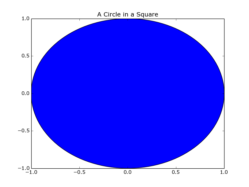
Let’s draw a square of side length 2r and a circle centred exactly in the middle of the square with radius r. A well organised blogger would show you a diagram of this set-up, screw it, this is the code to do it and this is what it looks like:

import matplotlib.pyplot as plt
fig = plt.figure()
axis = fig.add_subplot(1,1,1)
circle = plt.Circle((0,0), 1)
axis.add_patch(circle)
axis.set_xlim([-1,1])
axis.set_ylim([-1,1])
axis.set_title('A Circle in a Square')
plt.show()

A Circle in a Square

Brilliant – was it worth it? Probably not. But there you have it – with that set up we can now start the Monte Carlo bit. We’ll throw darts at that picture randomly; you’d expect the number of darts in the circle to be proportional to the area of the circle and the number of darts in the square to be proportional to the area of the square. Using that fact and the formulae for the areas of a circle and a square you can estimate Pi using the ratio of darts in the circle and in the square.

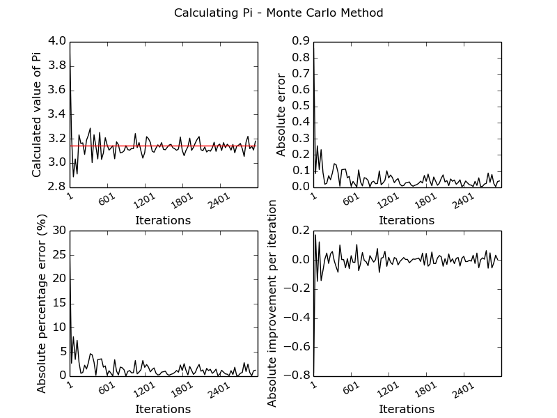
Sound good? It’s fairly easy to run this in Python and graph the output using Matplotlib. You’ll see I’ve used Object Oriented Python for this particular exercise, I don’t really know why. Especially because I had a chance to use inheritance and didn’t. Well done me. I’ve let everybody down. Anyway – this is the code I came up with and the graph below shows what I ended up with:

#!/usr/bin/python

import numpy as np
import math
import matplotlib.pyplot as plt

"""
Calculate pi using Monte-Carlo Simulation
"""

"""
First - the maths:
A circle has area Pi*r^2
A square wholly enclosing above circle has area 4r^2
If we randomly generate points in that square we'd expect the ratio of points in the square/points in the circle to equal the area of the square divided by the circle.
By that logic n_in_sq/n_in_cir = 4/Pi and so Pi = (4 * n_in_cir)/n_in_sq
"""

class pi_calculator(object):

    def __init__(self, radius, iterations):
        self.radius = radius
        self.iterations = iterations
        self.square = square(radius)
        self.circle = circle(radius)

    def scatter_points(self):
        for _ in range(self.iterations):
            point_x, point_y = ((2*self.radius) * np.random.random_sample(2)) - self.radius
            self.square.increment_point_count(point_x, point_y)
            self.circle.increment_point_count(point_x, point_y)

    def return_pi(self):
        return (4.0*self.circle.return_point_count())/self.square.return_point_count()

    def calculate_accuracy(self, calc_pi):
        absolute_error = math.pi - calc_pi
        percent_error = 100*(math.pi - calc_pi)/math.pi
        return (absolute_error, percent_error)

    def return_iterations(self):
        return self.iterations

class square(object):

    def __init__(self, radius):
        self.radius = radius
        self.lower_x = -radius
        self.lower_y = -radius
        self.upper_x = radius
        self.upper_y = radius
        self.point_count = 0


    def in_square(self, point_x, point_y):
        return (self.upper_x > point_x > self.lower_x) and (self.upper_y > point_y > self.lower_y)


    def increment_point_count(self, point_x, point_y, increment = 1):
        if self.in_square(point_x, point_y):
            self.point_count += increment

    def return_point_count(self):
        return self.point_count

class circle(object):

    def __init__(self, radius):
        self.radius = radius
        self.point_count = 0

    def in_circle(self, point_x, point_y):
        return point_x**2 + point_y**2 < self.radius**2

    def increment_point_count(self, point_x, point_y, increment=1):
        if self.in_circle(point_x, point_y):
            self.point_count += increment

    def return_point_count(self):
        return self.point_count


if __name__ == '__main__':
    axis_values = []
    pi_values = []
    absolute_error_values = []
    percent_error_values = []
    for _ in range(1,3000,30):
        pi_calc = pi_calculator(1, _)
        pi_calc.scatter_points()
        print "Number of iterations: %d    Accuracy: %.5f" % (pi_calc.return_iterations(), math.fabs(pi_calc.calculate_accuracy(pi_calc.return_pi())[0]))
        axis_values.append(_)
        pi_values.append(pi_calc.return_pi())
        absolute_error_values.append(math.fabs(pi_calc.calculate_accuracy(pi_calc.return_pi())[0]))
        percent_error_values.append(math.fabs(pi_calc.calculate_accuracy(pi_calc.return_pi())[1]))

    improvement_per_iteration = [absolute_error_values[index] - absolute_error_values[index-1] for index, value in enumerate(absolute_error_values) if index > 0]
    fig = plt.figure()
    fig.suptitle('Calculating Pi - Monte Carlo Method')
    ax1 = fig.add_subplot(2,2,1)
    ax2 = fig.add_subplot(2,2,2)
    ax3 = fig.add_subplot(2,2,3)
    ax4 = fig.add_subplot(2,2,4)
    plt.subplots_adjust(wspace=0.3, hspace=0.3)
    ax1.set_xticklabels([str(entry) for entry in axis_values[::len(axis_values)/5]], rotation=30, fontsize='small')
    ax1.set_xlabel('Iterations')
    ax1.set_ylabel('Calculated value of Pi')
    ax1.plot(pi_values, 'k')
    ax1.plot([math.pi for entry in axis_values], 'r')
    ax2.set_ylabel('Absolute error')
    ax2.set_xticklabels([str(entry) for entry in axis_values[::len(axis_values)/5]], rotation=30, fontsize='small')
    ax2.set_xlabel('Iterations')
    ax2.plot(absolute_error_values, 'k', label="Total Error")
    ax3.set_ylabel('Absolute percentage error (%)')
    ax3.set_xticklabels([str(entry) for entry in axis_values[::len(axis_values)/5]], rotation=30, fontsize='small')
    ax3.set_xlabel('Iterations')
    ax3.plot(percent_error_values, 'k', label="Percent Error")
    ax4.set_ylabel('Absolute improvement per iteration')
    ax4.set_xticklabels([str(entry) for entry in axis_values[::len(axis_values)/5]], rotation=30, fontsize='small')
    ax4.set_xlabel('Iterations')
    ax4.plot(improvement_per_iteration, 'k', label="Absolute change")
    plt.savefig('pi_calculation.png')
    plt.show()

giving us:

Monte Carlo estimation of Pi – an Investigation

I can only apologise for any dodgy code in there – in my defence, it was early in the morning. As you can see, it only takes around 100 ‘darts thrown at the board’ to start to see a reasonable value for Pi. I ran it up to about 10,000 iterations without hitting any significant calculation time. The fourth graph doesn’t really show anything interesting – I just couldn’t think of anything to put there.

That’ll do for now – I built something that’ll stream tweets on the Scottish Independence Referendum but don’t know what to do with it yet; there’ll likely be some sort of blog post. There’s a chance I’ll do some sentiment analysis but I’m not sure yet.

When you play the Game of Thrones, you win or you die.