Hey all,
So from that long list I posted I’ve decided I’m most interested in the fastest growing and falling towns in the UK, as measured by the average house selling price. Once we’ve got a bunch of hot/not towns we might even be able to have a look at what these towns looked like before their boom. The hope is then that we’ll be able to find towns in that situation right now and boom, we’re housing moguls.
Given my poor excuse for hardware, we’ll have to start in bash:
awk -F, '{print $3"-"$4"-"($(NF-3))}' pp-all.csv | tr -d '"' | cut -d '-' -f1,2,3,5 | tr '-' 't' | awk '{summary_array[$2"-"$3"-"$4] += $1; count_array[$2"-"$3"-"$4]++} END {for (region in summary_array) print region"t"summary_array[region]/count_array[region]}' | tr '-' 't' | sort -nk1 -nk2 > average_sale_price_by_town_and_month.txt
where pp-all.csv is all the UK housing data as downloaded from data.gov.uk. The format of the data and what the above code does is inferrable from the following R code:
library(reshape2)
library(plyr)
library(ggplot2)
myData <- read.csv('average_sale_price_by_town_and_month.txt', header=F, sep='t')
colnames(myData) <- c("Year", "Month", "Town", "Average_Price")
## Let's not make the same mistakes as we did last time - which data should we remove pre-analysis?
summary(count(myData, c('Town'))$freq)
## From that, I'm going to say let's remove any town without 229 points.
myData <- myData[!(myData$Town %in% levels(myData$Town)[(count(myData, c('Town'))$freq < 229)]),]
I’m going to break out of code mode to explain that last line because it is horrible. I’m first grouping my data by town and counting the number of entries – in SQL this’d be SELECT count(date) FROM myData GROUP BY Town . I’m then comparing every entry in the list to 229 (the max number of points each town can have) and producing a logical list of the same size as the number of towns indicating whether the town at that index has a full complement of points. levels(myData$Town) gives me a list of all the towns which is placed against the previously calculated logical list – only towns matching a TRUE are kept. At that point, we’ve got a list containing all the towns we want to keep – myData$Town %in% compares the Town column of myData against this list and acts like a SQL where clause. Finally, in confusing developments, I’ve inverted all of the above logic with an ! – this’ll now only keep columns where the number of entries per town is greater than 228. The comma before the square bracket says to include all columns (we could add filters there if we liked). We assign all of this to itself, in effect filtering the original data frame by removing any lines belonging to towns which don’t have a full complement of points. All in that one line.
In practical advice for the novice R coder (which I’d class myself as) – start with the smallest bit of code you can and then add bits on when you’re comfortable with what they’re doing. Actually, that’s not just true of R – the bash one-liner above would likely be best constructed in exactly the same way.
Anyway, where were we?
myData$Datey <- as.Date(paste(myData$Year, myData$Month, 1, sep='-'), '%Y-%m-%d')
myData <- myData[,!(names(myData) %in% c("Year", "Month"))]
ts_frame <- dcast(myData, Datey ~ Town, value.var="Average_Price")
row.names(ts_frame) <- ts_frame$Datey
ts_frame <- ts_frame[,!(names(ts_frame) %in% c("Datey"))]
growth_frame = data.frame(matrix(0, ncol=1, nrow=length(ncol(ts_frame))))
row.names(growth_frame) <- names(ts_frame)
for (i in 1:ncol(ts_frame)) {
  total_growth <- 100*((ts_frame[length(ts_frame[,i]),i] - ts_frame[1,i])/ts_frame[1,i])
  growth_frame[[names(ts_frame)[i]]] = total_growth
}
long_growth_frame <- melt(growth_frame)
colnames(long_growth_frame) <- c("Town", "Percentage_growth")
long_growth_frame <- long_growth_frame[long_growth_frame$Percentage_growth > 0.1,]
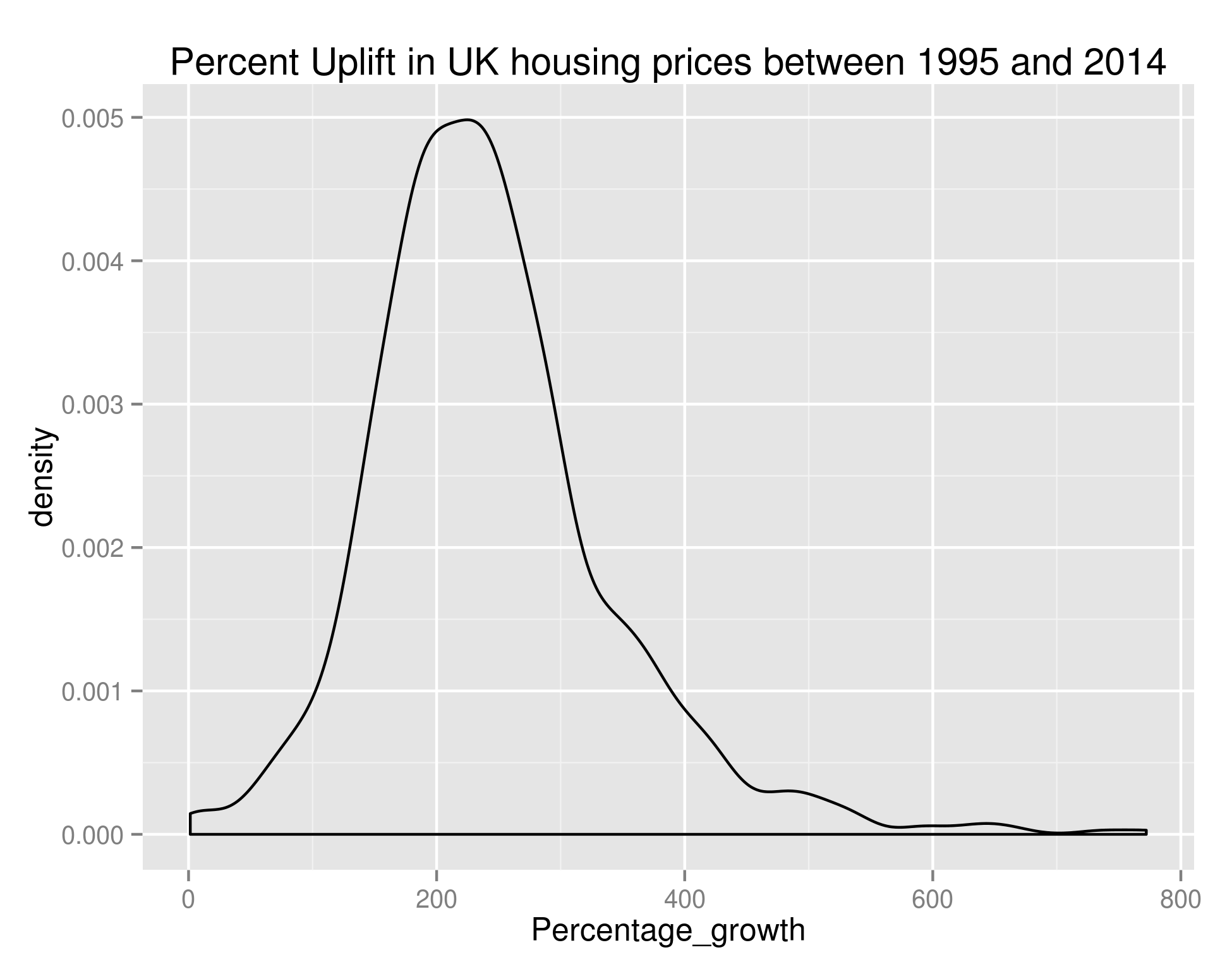
ggplot(long_growth_frame, aes(x=Percentage_growth)) + geom_density() + ggtitle("Percent Uplift in UK housing prices between 1995 and 2014")
giving us:
As we can see, the bulk of towns experienced between 100% and 400% growth in that time – if anybody can point me towards UK salary figures over that time period I think that’d be a nice set to join this with.
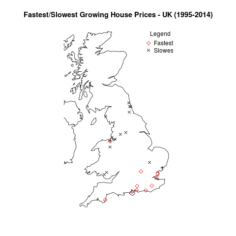
Anyway, let’s take what we’ve done in the previous post on house prices and plot the data on a UK map. There are too many points for me to reasonably plot all of them – let’s go with the top 20 (Red diamonds) and bottom 20 (black crosses):
ordered_growth_frame <- long_growth_frame[order(long_growth_frame$Percentage_growth),]
library(maps)
library(mapdata)
library(RCurl)
library(RJSONIO)
## A couple of functions allowing us to dynamically get the longitude and latitude of regions
construct.geocode.url <- function(address, return.call = "json", sensor = "false") {
  root <- "http://maps.google.com/maps/api/geocode/"
  u <- paste(root, return.call, "?address=", address, "&sensor=", sensor, sep = "")
  return(URLencode(u))
}

gGeoCode <- function(address,verbose=FALSE) {
  if(verbose) cat(address,"n")
  u <- construct.geocode.url(address)
  doc <- getURL(u)
  x <- fromJSON(doc,simplify = FALSE)
  if(x$status=="OK") {
    lat <- x$results[[1]]$geometry$location$lat
    lng <- x$results[[1]]$geometry$location$lng
    return(c(lat, lng))
  } else {
    return(c(NA,NA))
  }
}

map('worldHires',  c('UK', 'Ireland', 'Isle of Man','Isle of Wight'), xlim=c(-7,2), ylim=c(50.1,58.7))
long_and_lat <- data.frame(sapply(paste(head(ordered_growth_frame, n=20)$Town, ", UK", sep=''), function(x) gGeoCode(x)))
row.names(long_and_lat) <- c("Latitude", "Longitude")
long_and_lat <- data.frame(t(long_and_lat))
points(long_and_lat$Longitude, long_and_lat$Latitude, col=1, pch=4)
long_and_lat <- data.frame(sapply(paste(tail(ordered_growth_frame, n=20)$Town, ", UK", sep=''), function(x) gGeoCode(x)))
row.names(long_and_lat) <- c("Latitude", "Longitude")
long_and_lat <- data.frame(t(long_and_lat))
points(long_and_lat$Longitude, long_and_lat$Latitude, col=2, pch=5)
title('Fastest/Slowest Growing House Prices - UK (1995-2014)')
legend("topright", legend=c("Fastest", "Slowest"), title="Legend", bty="n", pch=c(5,4), col=c("red", "black"), inset=c(-0.05,0))
giving us:
So it looks like the South Coast has been the place to buy houses in the last 20 or so years. And the North East/North West were the places to be avoided.
OK – that’s all well and good but it doesn’t really tell us anything about the area we should be buying houses in now. Hold your horses. I’m getting to that. Obviously we’re not really going to be able to learn anything looking at the price difference between the end of our ‘test’ period and the start of our ‘test’ period. We need to build our model over a subset of this data, and test it against the remaining data.
For my next trick (blog post) I’ll look at predicting the fastest growing regions. As a sneak peek, to do we’ll use growth % as the metric we’re trying to predict (a continuous variable) and we’ll create features out of the input data set. I don’t know which method we’ll use yet but it’ll be one of linear regression, SVM regression or neural networks. Likely whichever is best supported by the language I choose to use. I’ve used Libsvm before and found it very good so maybe that.
What we do in life echoes in eternity.

