clustering – DogDogFish

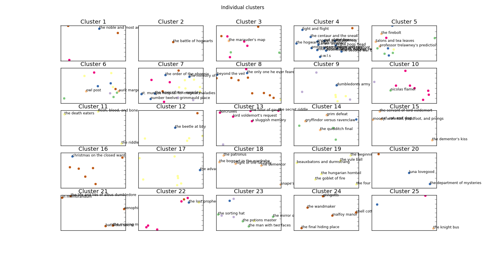
I’ll open up with the money-shot – these are all of the clusters that I was able to find using the whole Harry Potter and grouping by chapter:

Every cluster plotted separately.

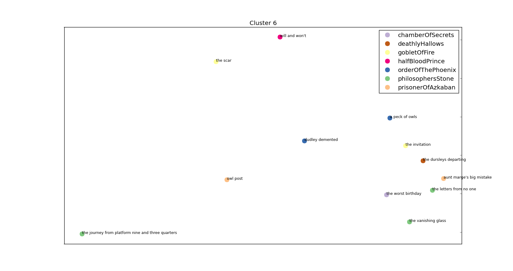
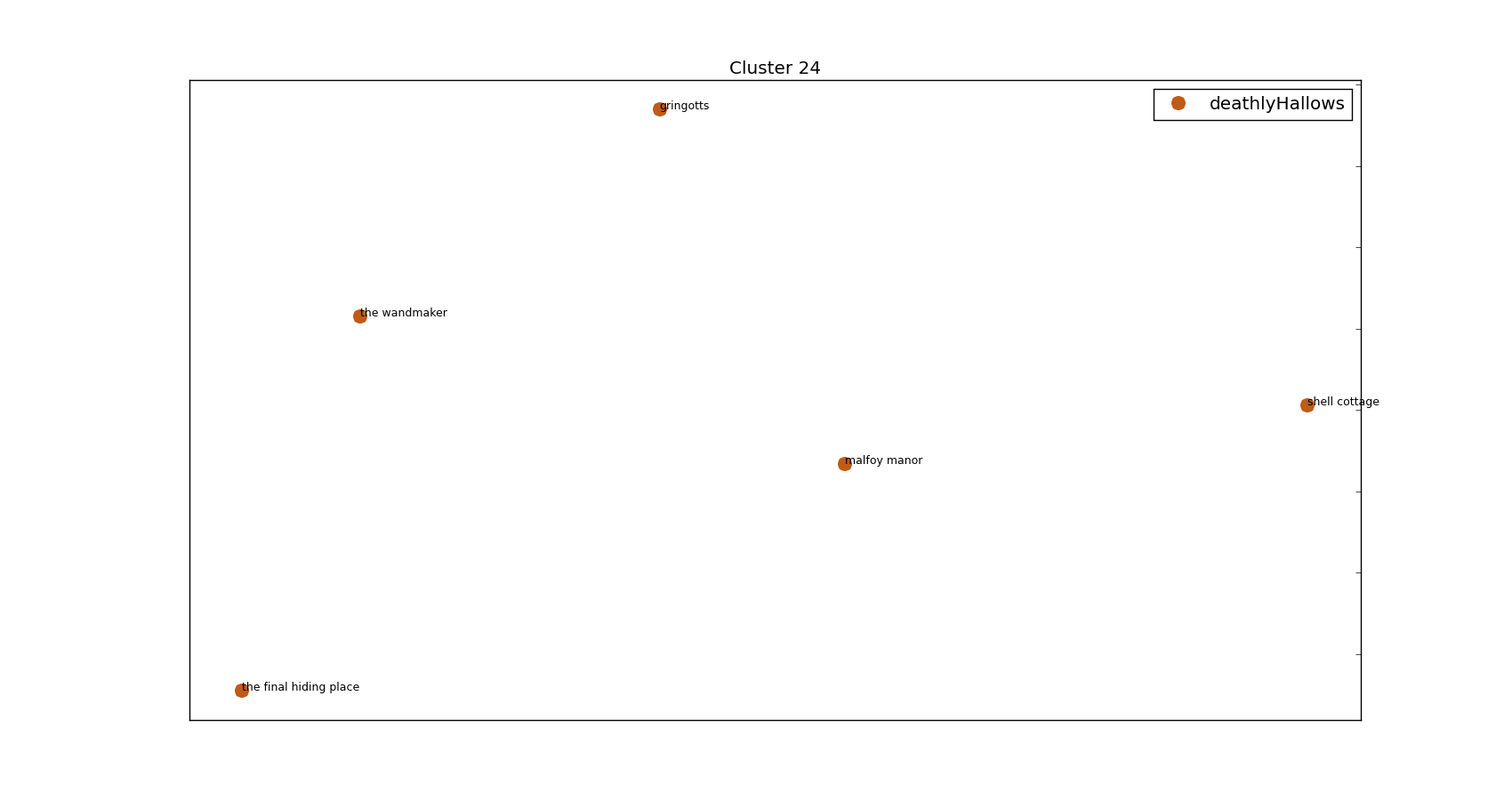
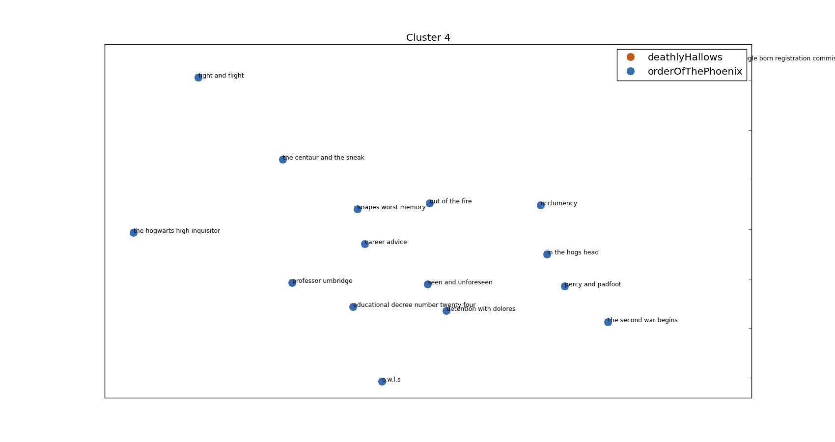
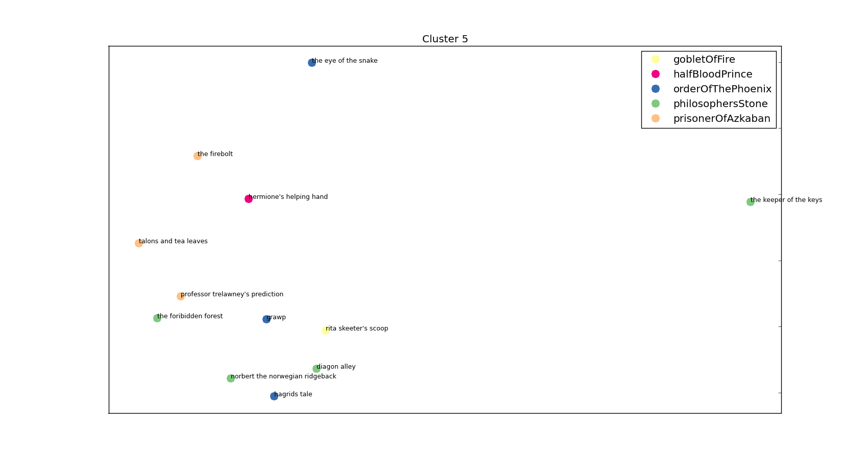
That’s far too messy to be of any practical use so let’s have a look at a couple of those clusters in more detail:

One of the clusters – a Dursley/Privet Drive heavy cluster!

and

This is a pretty Griphook/Goblin heavy cluster featured on the storyline in book 7.

Hopefully that’s piqued your interest enough to continue on scrolling and see how we got these clusters – and see the words that tie them all together! The code for generating these is on my Github (https://github.com/Kali89/HarryPotterClusters) and all the graphs and documents are contained there.

I went to a really interesting talk at PyData that was about Latent Dirichlet Allocation, a topic entirely new to me. I thought I’d love to apply it to my favourite book series – Harry Potter. However, that didn’t happen…instead you get this. A heavy rip off of an excellent post (http://brandonrose.org/clustering) that walks through how to cluster documents using a bunch of techniques including K-Means.

Step 1

Get plain text copies of all the Harry Potter books and make sure they’re all formatted in roughly the same way. As is often the case, this step took bloody ages.

Step 2

I want a few different documents – more than 7 (the number of Harry Potter books for the heathens out there) but substantially less than the number of sentences in all 7 books. Treating each chapter as a separate document seemed to make most sense and so here I initialise everything I need and split my books into chapter.

So at this point we’ve nicely got ourselves a list of chapter titles and a list of the associated text (as a string).

Step 3

Now we’ve got our chapters we’re going to want to tokenise the text in them. Basically this means converting a string into discrete tokens – what we’d think of as words. The reason it’s got a fancy name and I’m being a bit careful about my terminology is because tokenisation also takes care of things like punctuation and isn’t as simple as just splitting a string into separate words. Having said that, I’ve basically taken the path of least resistance and so have gone with a very simple tokenisation scheme. I’m also going to skip over the pain of utf-8 encoding/decoding/recoding. I’ve basically just dropped any character that I’ve found in the least bit complicated.

Step 4

Next I’m going to perform TF-IDF on my chapters. Here, I convert each token into a number and look at how many times that token appears in a given document, and how many documents that token appears in overall. So in this instance I’m looking to see how often a given word appears in this particular chapter and in how many chapters throughout all 7 books the token appears in. This gives us an idea of how important/prominent a word is in a given chapter, taking into account how common the word is throughout all the chapters. As an example ‘Harry’ is likely to feature a lot in a given chapter but also is likely to feature in every chapter and so probably isn’t especially important to any given chapter’s classification. ‘Nicolas Flamel’, however, is going to appear a reasonable amount in a few chapters but not at all in all the rest. We therefore know that Nicolas Flamel is important in the chapters he does appear in.

Luckily, I don’t have to worry about the implementation of TF-IDF – sklearn has got it.

This gives me a large sparse matrix with the TF-IDF score for each word in each document as the entries. If you pay close attention to the parameters I’ve passed along to TfidfVectorizer as they are ripe for the changing. Firstly, `max_df=0.75` is saying that I don’t care about words that appear in more than 75% of the chapters. `min_df=0.05` is saying that I don’t care about words that appear in fewer than 5% of chapters. You can see I passed along my tokeniser and that I’m using English stop-words (that is, I’m removing the most common English words). Finally, I’m generating n-grams between 1 and 4.

For those uninitiated with n-grams they’re basically a way of splitting text up into handy little chunks. As an example, 3-grams of the following sentence:

“This is not the greatest song in the world”

would be:

“This is not”, “is not the”, “not the greatest”, “the greatest song”, e.t.c.

This allows me to pick out common phrases such as “Snape said” and “wizarding world”. Again, that’s a setting that is begging to be played about with.

Step 5

Performing K-means clustering we get output like so:

Cluster 18 words: Top words: maxime,madame maxime,karkaroff,madame,hagrid,cedric,moody,krum,champions,tournament

Chapter: the hungarian horntail, Book: gobletOfFire Chapter: the goblet of fire, Book: gobletOfFire Chapter: the four champions, Book: gobletOfFire Chapter: beauxbatons and durmstrang, Book: gobletOfFire Chapter: the beginning, Book: gobletOfFire Chapter: the yule ball, Book: gobletOfFire

which is obviously quite a handy little cluster. It’s successfully managed to only take chapters from one book (given that we’ve not allowed K-means access to the book information that is a bit of a triumph). For those aware of Harry Potter you’ll see this is a Triwizard Tournament heavy cluster. Another example:

Cluster 10 words: Top words: wormtail,cold voice,voldemort,lord,cauldron,riddle,cedric,man,master,faithful


Chapter: the riddle house, Book: gobletOfFire

Chapter: flesh, blood, and bone, Book: gobletOfFire

Chapter: the death eaters, Book: gobletOfFire

Again, all the clusters are from one book – I’m counting that as a result. Added bonus, they’re not sequential chapters! I happen to know (by being a massive Harry Potter geek) that these chapters are towards the start and end of book 4 and focus heavily on Voldemort and Peter Pettigrew.

So far so good and in fact I could stop here but wouldn’t it be nice to visualise those clusters so we can see the topics we’ve picked out graphically? Even if you said no then it doesn’t really matter. I’m still going to do it.

Step 6

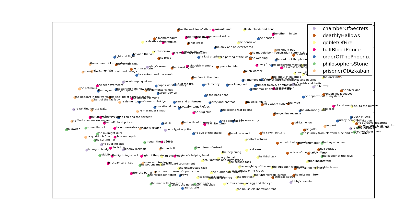
First things first, let’s plot all of the chapters on one graph and colour code them with the book from which they came. It’s not a great way of visualising clusters but it is a great way of seeing how everything is laid out:

A messy picture of all the chapters projected into 2d space.

Again, this section is shamelessly copied from the aforementioned blog but ultimately we’re projecting the cosine differences between the tf-idf matrix terms into 2-dimensional space. I declare a colour dictionary for each of the books and then rattle through the chapters plotting them.
I’m sure you’ll agree that’s far too messy for anybody to really do anything with. If you’re following along with the code you’ll see that next I generate the subplot figure shown at the top.

Finally, I create plots for each of the clusters – a few examples of which are:

Cluster 3 words: Top words: umbridge,professor,dont,professor umbridge,snape,sirius,im,said hermione,harrys,youre


Chapter: the muggle born registration commission, Book: deathlyHallows

Chapter: the hogwarts high inquisitor, Book: orderOfThePhoenix

Chapter: o.w.l.s, Book: orderOfThePhoenix

Chapter: the second war begins, Book: orderOfThePhoenix

Chapter: educational decree number twenty four, Book: orderOfThePhoenix

Chapter: the centaur and the sneak, Book: orderOfThePhoenix

Chapter: percy and padfoot, Book: orderOfThePhoenix

Chapter: detention with dolores, Book: orderOfThePhoenix

Chapter: occlumency, Book: orderOfThePhoenix

Chapter: in the hogs head, Book: orderOfThePhoenix

Chapter: out of the fire, Book: orderOfThePhoenix

Chapter: professor umbridge, Book: orderOfThePhoenix

Chapter: fight and flight, Book: orderOfThePhoenix

Chapter: seen and unforeseen, Book: orderOfThePhoenix

Chapter: career advice, Book: orderOfThePhoenix

Chapter: snapes worst memory, Book: orderOfThePhoenix

generates:

Umbridge’s cluster

Everybody’s favourite professor – Dolores Umbridge!

And another:


Top words: hagrid,yeh,ter,said hagrid,professor,said hermione,malfoy,o,professor trelawney,trelawney
Chapter: professor trelawney's prediction, Book: prisonerOfAzkaban

Chapter: talons and tea leaves, Book: prisonerOfAzkaban

Chapter: the firebolt, Book: prisonerOfAzkaban

Chapter: diagon alley, Book: philosophersStone

Chapter: the foribidden forest, Book: philosophersStone

Chapter: the keeper of the keys, Book: philosophersStone

Chapter: norbert the norwegian ridgeback, Book: philosophersStone

Chapter: hagrids tale, Book: orderOfThePhoenix

Chapter: the eye of the snake, Book: orderOfThePhoenix

Chapter: grawp, Book: orderOfThePhoenix

Chapter: hermione's helping hand, Book: halfBloodPrince

Chapter: rita skeeter's scoop, Book: gobletOfFire

and visually:

Keeper of the Keys

The anti-Umbridge – it’s Hagrid’s cluster!

I’ll stop on the random copy/pasting of the clusters and stick them all on my Github – I think you’ve got the idea! All in all I’m pretty happy with how this has worked but I am very dependent on individual character names. I tried just looking at 2-grams but it usually just gave me ” said” with a few exceptions (‘wizarding world’, ‘said softly’, ‘death eater’, ‘godrics hollow’). I’ve also put almost zero effort into formatting the images – you know roughly what it’s meant to look like: having the pictures look good is an exercise I’m leaving to the reader’s imagination.

There’s loads more stuff I could do but I’m going to eat a chicken and go swimming so it’ll have to wait.

All was well.

Hi all,

Bit of a different blog coming up – in a previous post I used Markov Clustering and said I’d write a follow-up post on what it was and why you might want to use it. Well, here I am. And here you are. So let’s begin:

In the simplest explanation, imagine an island. The island is connected to a whole bunch of other islands by bridges. The bridges are made out of bricks. Nothing nasty so far – apart from the leader of all the islands. They’re a ‘man versus superman’, ‘survival of the fittest’ sort and so one day the issue a proclamation. “Every day a brick will be taken from every bridge connected to your island and the bricks will be reapportioned on your island back to the bridges, in proportion to the remaining number of bricks in the bridge.”

At first, nobody is especially worried – each day, a brick disappears and then reappears on a different bridge on the island. Some of the islands notice some bridges getting three or four bricks back each day. Some hardly ever seem to see a brick added back to their bridge. Can you see where this will lead in 1000 years? In time, some of the bridges (the smallest ones to start off with) fall apart and end up with no bricks at all. If this is the only way between two islands, these islands become cut off entirely from each other.

This is basically Markov clustering.

For a more mathematical explanation:

Let’s start with a (transition) matrix:

import numpy as np
transition_matrix = np.matrix([[0,0.97,0.5],[0.2,0,0.5],[0.8,0.03,0]])

$Transition Matrix = begin{matrix} 0 & 0.97 & 0.5 \ 0.2 & 0 & 0.5 \ 0.8 & 0.03 & 0 end{matrix}$

In the above ‘islands’ picture those numbers represent the number of bricks in the bridges between islands A, B and C. In the random-walk interpretation, those are the probabilities that you’ll end up at each node as the number of random walks tends to infinity. In my previous post on house prices, I used a correlation matrix.

First things first – I’m going to stick a one in each of the identity areas. If you’re interested in why that is, have a read around self-loops and, even better, try this out both with and without self-loops. It sort of fits in nicely with the above islands picture but that’s more of a fluke than anything else – there’s always the strongest bridge possible between an island and itself. The land. Anyway…

np.fill_diagonal(transition_matrix, 1)

$Transition Matrix = begin{matrix} 1 & 0.97 & 0.5 \ 0.2 & 1 & 0.5 \ 0.8 & 0.03 & 1 end{matrix}$

Now let’s normalize – make sure each column sums to 1:

transition_matrix = transition_matrix/np.sum(transition_matrix, axis=0)

$Transition Matrix = begin{matrix} 0.5 & 0.485 & 0.25 \ 0.1 & 0.5 & 0.25 \ 0.4 & 0.015 & 0.5 end{matrix}$

Now we perform an expansion step – that is, we raise the matrix to a power (I’ll use two – you can change this parameter – in the ‘random-walk’ picture this can be thought of as varying how far a person can walk from their original island).

transition_matrix = np.linalg.matrix_power(transition_matrix, 2)

$Expanded Matrix = begin{matrix} 0.3985 & 0.48875 & 0.37125 \ 0.2 & 0.30225 & 0.275 \ 0.4015 & 0.209 & 0.35375 end{matrix}$

Then we perform the inflation step – This involves multiplying each element in the matrix by itself (to a power) and then normalizing on column again. Again, I’ll be using two as a power – increasing this leads to a greater number of smaller clusters:

for entry in np.nditer(transition_matrix, op_flags=['readwrite']):
    entry[...] = entry ** 2

$Inflated Matrix = begin{matrix} 0.15880225 & 0.23887556 & 0.13782656 \ 0.04 & 0.09135506 & 0.075625 \ 0.16120225 & 0.043681 & 0.12513906 end{matrix}$

Finally (for this iteration) – we’ll normalize by row.

transition_matrix = transition_matrix/np.sum(transition_matrix, axis=0)

$Normalized Matrix = begin{matrix} 0.44111185 & 0.63885664 & 0.40705959 \ 0.11110972 & 0.24432195 & 0.22335232 \ 0.44777843 & 0.11682141 & 0.36958809 end{matrix}$

And it’s basically that simple. Now all we need to do is rinse and repeat the expansion, inflation and normalization until we hit a stable(ish) solution i.e.

$Normalized Matrix_{n+1} - Normalized Matrix_n < epsilon$
for some small epsilon.

Once we’ve done this (with this particular matrix) we should see something like this:

$Final Matrix = begin{matrix} 1 & 1 & 1 \ 0 & 0 & 0 \ 0 & 0 & 0 end{matrix}$

Doesn’t look like a brilliant result be we only started with a tiny matrix. In this case we have all three nodes belonging to one cluster. The first node (the first row) is the ‘attractor’ – as it has values in its row it is attracting itself and the second and third row (the columns). If we were to end up with the following result (from a given initial matrix):

$Final Matrix = begin{matrix} 1 & 0 & 1 & 0 & 0\ 0 & 1 & 0 & 1 & 0\ 0 & 0 & 0 & 0 & 0\ 0 & 0 & 0 & 0 & 0\ 0 & 0 & 0 & 0 & 1\ end{matrix}$

This basically says that we have three clusters {1,3} (with 1 as the attractor), {2,4} (with 2 as the attractor) and {5} on its lonesome.

Instead of letting you piece all that together here’s the code for Markov Clustering in Python:

import numpy as np
import math
## How far you'd like your random-walkers to go (bigger number -> more walking)
EXPANSION_POWER = 2
## How tightly clustered you'd like your final picture to be (bigger number -> more clusters)
INFLATION_POWER = 2
## If you can manage 100 iterations then do so - otherwise, check you've hit a stable end-point.
ITERATION_COUNT = 100
def normalize(matrix):
    return matrix/np.sum(matrix, axis=0)

def expand(matrix, power)
    return np.linalg.matrix_power(matrix, power)

def inflate(matrix, power):
    for entry in np.nditer(transition_matrix, op_flags=['readwrite']):
        entry[...] = math.pow(entry, power)
    return matrix

def run(matrix):
    np.fill_diagonal(matrix, 1)
    matrix = normalize(matrix)
    for _ in range(ITERATION_COUNT):
        matrix = normalize(inflate(expand(matrix, EXPANSION_POWER), INFLATION_POWER))
    return matrix

If you were in the mood to improve it you could write something that’d check for convergence for you and terminate once you’d achieved a stable solution. You could also write a function to perform the cluster interpretation for you.

As you were.

Tag: clustering

Finding Topics in Harry Potter using K-Means Clustering.

Markov Clustering – What is it and why use it?

Bloggers

Subscribe to Blog via Email

Recent Posts

Categories