Hi All,
After work over one year (approximately 800,000 data points) it’s time to start ramping things up a bit and we’ll be heading into the realms of big data. There are a bunch of definitions of big data floating around but I’m going to go with the one I like the most: “Big data is the point at which the size of your data becomes part of the problem.” That of course depends entirely on the hardware you’ve got and given my current hardware situation, as soon as we start looking at multiple years of house sale data, we’re firmly in ‘big data’ territory. In fact, the size of the data isn’t really that large – only ~20 million rows with a total size of 3.2GB. I could upgrade my RAM for a small amount and we’d be fine to deal with this in the usual ways. However, I’m cheap, the shops are closed and I’d rather think of a less hardware bound way of doing it.
Unfortunately for me, while working at home on my own projects, I don’t have access to any cluster of computers so won’t be throwing my data into HDFS and getting my mappers and reducers polished. At work we’re soon to be adding 40TB of storage and 10 more nodes to our existing cluster and that set up would chew through this sort of thing like nobody’s business. Given an i5 and 6GB of RAM, we’re going to have to be a tad more creative 😉 It’s also worth noting that, for 3.2GB of data, distributing the problem isn’t likely the most efficient solution. Just because I’m talking about big data, there’s no reason we can’t use R, Python, SQL or anything else that will solve the problem.
I liked what we were able to do in R and don’t feel I’ve had a sufficiently deep dive into the statistical functions it offers and so will be trying to use it again. Fitting all the data in memory isn’t going to work but R offers a number of packages for working with data that exceeds the RAM you’d be willing to give it; I’ll be using bigmemory.
First things first, all the data is split across text files. If we want to have them read into a single table I think we’ll be best creating that text file in bash and adding a new column with the year – bash to the rescue:
for file in pp-*.csv

do

echo "Processing $file...";

year=${file:3:4};

awk -F, -v year=$year '{print year","$0}' $file >> pp-all.csv;

done
At the risk of stating the obvious, that will loop over all the relevant files, extract the year from the title of the file, prepend it to the start of the line and then append the line to pp-all.
O.K – originally I was going to use bigmemory but have found it unsuitable for the task (namely, I couldn’t even get it to load the file from disk). I’m sure that’s more a damning indictment of my own ability rather than bigmemory but I’ll proceed in a different way for now.
cut -d ',' -f3,4 pp-all.csv | tr -d '"' | cut -d '-' -f1,2 | awk -F, '{ total_array[$2] += $1; count_array[$2] += 1} END {for (region in total_array) print region"t"total_array[region]/count_array[region]}' | tr '-' ' ' | sort -nk1 -nk2 | sed -e 's/s+/-/' > price_summary_by_month.txt
OK – it’s a bit of a nasty one-liner but it basically:
1.) Gets the date and house sale price
2.) Formats the output
3.) Create an array of the count and sum of sale prices per month
4.) Sort by date and format
5.) Output to price_summary_by_month.txt
Now I’ve got myself a lovely text file – I decided to have a dig into Python and especially, Matplotlib. As it’s not really relevant to the overall direction of this analysis I won’t include the code here but it’s available on my Github. As a summary, this script looks at the percentage of total value of the year’s sales made in each month. A vector is built for each month and then the Gaussian density is calculated for that month. This is plotted versus the surrounding months. I’m aware that’s likely a poor explanation but if you’re interested, have a look at the code and feel free to drop me a comment. The output is something like this:
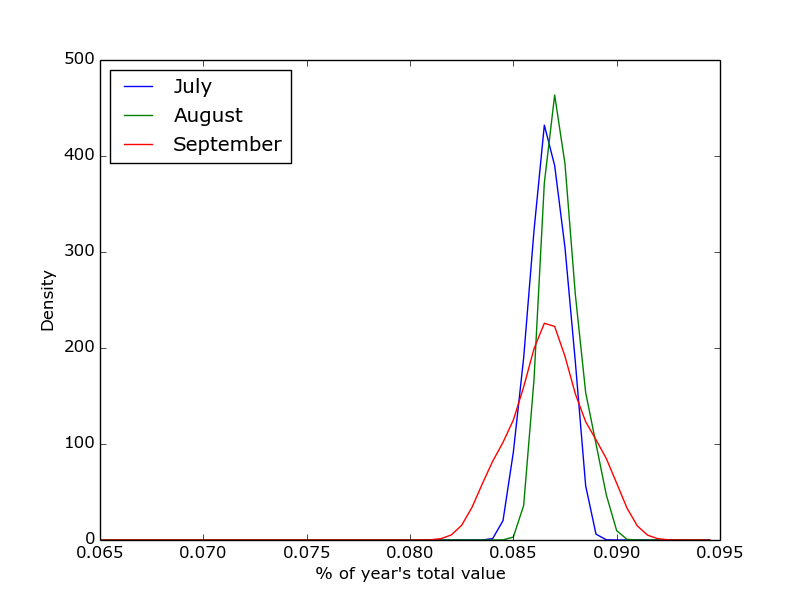
% of value of house sales since 1995, by month.
Anyway, back to the main thread of the investigation. I’ve got a relatively small time-series and I’m investigating the periodicity of the data – I’m right back in native R territory.
priceSummary <- read.table('price_summary_by_month.txt', header=F, col.names=c("date", "price"))
pricetimeseries <- ts(priceSummary$price, frequency=12, start=c(1995,1))
plot(pricetimeseries, ylab="Average sale price (£)", main="UK House Prices")
Giving us:
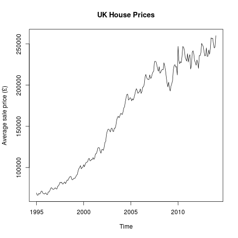
Average UK House Price (by month)
That’s pretty much as you’d expect – generally rising prices with a bit of a wobble around the housing crash. Disappointingly, there doesn’t seem to be that much evidence of seasonality being a factor. However, R provides us the tools to see whether or not that’s the case:
library(ggplot2)
library(scales)
pricetimeseriescomponents <- decompose(pricetimeseries)
plot(pricetimeseriescomponents)
seasonality <- data.frame(pricetimeseriescomponents$seasonal[c(1:12)])
seasonality$Month <- factor(month.name, levels=month.name)
colnames(seasonality) <- c("Price", "Month")
ggplot(seasonality, aes(x=Month, y=Price)) + geom_bar(stat="identity") + ggtitle("Seasonal variations in house sale price") + theme(axis.text.x = element_text(angle=90, hjust=1)) + scale_y_continuous(name="Price difference (£)", labels=comma)
orderedSeasonality <- transform(seasonality, Month = reorder(Month, Price))
ggplot(orderedSeasonality, aes(x=Month, y=Price)) + geom_bar(stat="identity") + ggtitle("Seasonal variations in house sale price") + theme(axis.text.x = element_text(angle=90, hjust=1)) + scale_y_continuous(name="Price difference (£)", labels=comma)
This gives us our first hint at some real cyclicity to the housing market:
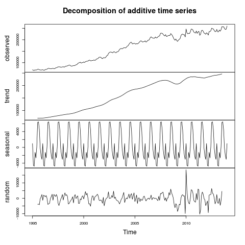
Decomposition of UK House Prices
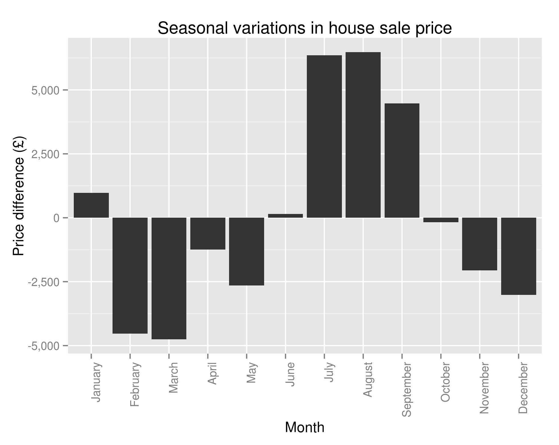
Seasonality of House Prices – the amount above/below average you’ll pay for a house based on the month
and a perhaps more helpful, sorted version:
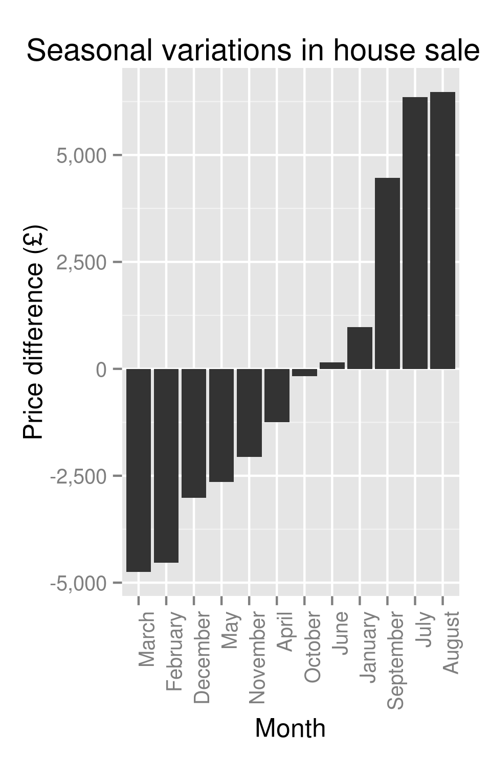
Ordered seasonality of House Prices – the amount above/below average you’ll pay for a house based on the month
Well well well. Time to throw the cowboy hat into the air, unholster our pistol and start firing wildly into the sky? Or at least quietly inform those who I know who are looking to buy/sell a house that they can likely save/make themselves an extra £10,000 or so if only they’re willing to wait until summer before selling?
Unfortunately, I’m not confident enough to say that just yet. I’ve already fairly conclusively shown that there are a bunch of factors that affect the sale price of a house. Now while I’m happy to say that the month of the year is significant in determining the sale price, I don’t really know why. It could be that people are more inclined to buy houses in the south during summer. As these houses are more expensive, we see the average house price rise in the summer months. It could be that people are less inclined to buy terraced houses during the summer (heating concerns?) and, as terraced houses are generally cheaper, the average sale price is inflated.
If either of those statements, or indeed, any other like it that I’ve not thought of are true it could lead to me giving bad advice in specific cases. To be able to report anything especially useful (and ultimately, actionable) we’ll need to look a bit closer at the causes of seasonality. My next post will hopefully address these issues and will try to determine whether or not the average UK house buyer is better off waiting until winter before buying.
Could you upload the data source or part of the data source at some place?
Best.